Calling C from R: A Performance Tutorial

1. Introduction

In data analysis and statistical computing, R is an excellent language for its expressiveness and extensive statistical libraries. However, R can be slow for certain computationally intensive tasks. This is where calling C or C++ from R becomes valuable.

In this tutorial, we’ll explore:

Why we need to call C from R
When to use C instead of pure R
How to implement C functions using Rcpp
Real-world examples with performance comparisons

This tutorial builds on our previous kernel density estimation post, where we implemented algorithms in R. Now, we’ll see how to accelerate these computations using C.

2. Why Call C from R?

Performance Comparison

R is an interpreted language, which makes it flexible but slower for certain operations. C is a compiled language that runs much closer to the hardware, making it significantly faster for:

Loops: Especially nested loops or loops with millions of iterations
Numerical computations: Heavy mathematical calculations
Memory-intensive operations: When you need fine control over memory
Recursive algorithms: Where function call overhead matters

Speed gains: C can be 10x to 1000x faster than R for loop-heavy computations.

When to Use C from R

*Use C when:**

You have loops that iterate millions of times
You’re performing the same simple operation repeatedly
Profiling shows a specific R function is a bottleneck
You need numerical precision or memory efficiency
Existing R functions are too slow for your application

*Don’t use C when:**

Vectorized R code already runs fast enough
You’re doing exploratory data analysis
The bottleneck is I/O (reading/writing files)
The code complexity isn’t worth the speedup
R packages already provide optimized solutions

3. Getting Started with Rcpp

Installation

# Install Rcpp package
install.packages("Rcpp")

Your First C Function in R

Let’s start with a simple example: computing the sum of numbers from 1 to n.

library(Rcpp)

# Pure R version
sum_r <- function(n) {
  total <- 0
  for(i in 1:n) {
    total <- total + i
  }
  return(total)
}

# C++ version using Rcpp
Rcpp::cppFunction("
double sum_cpp(int n) {
  double total = 0.0;
  for(int i = 1; i <= n; ++i) {
    total += i;
  }
  return total;
}
")

# Test both versions
n <- 1000000
system.time(result_r <- sum_r(n))

   user  system elapsed 
  0.009   0.000   0.009

system.time(result_cpp <- sum_cpp(n))

   user  system elapsed 
  0.000   0.001   0.000

Key differences:

C++ requires type declarations (double, int)
Array indexing starts at 0 in C, 1 in R
C++ uses ++i for increment, R uses i + 1

4. Example 1: Alternating Series Convergence

Problem

Compute the alternating harmonic series: 1 - 1/2 + 1/3 - 1/4 + … = ln(2)

This is a good example because:

It requires a loop with millions of iterations
Each iteration is a simple calculation
It demonstrates convergence visualization

Implementation

# C function to compute first n terms
Rcpp::cppFunction("
double alt2(int n) {
  double total = 0.0;
  for(int i = 1; i <= n; ++i) {
    total += pow(-1.0, i + 1) / i;
  }
  return total;
}
")

# Test the function
cat("alt2(10) =", alt2(10), "\n")

alt2(10) = 0.6456349

cat("alt2(100) =", alt2(100), "\n")

alt2(100) = 0.6881722

cat("alt2(1000) =", alt2(1000), "\n")

alt2(1000) = 0.6926474

cat("alt2(1000000) =", alt2(1000000), "\n")

alt2(1000000) = 0.6931467

cat("ln(2) =", log(2), "\n")

ln(2) = 0.6931472

Visualization

# Create sequence of n values
n <- unique(c(
  seq(1, 100, by = 1),
  seq(105, 1000, by = 5),
  seq(1010, 10000, by = 10),
  seq(10050, 100000, by = 50),
  seq(100500, 1000000, by = 500)
))

# Compute values
alt2_vals <- sapply(n, alt2)
ln2 <- log(2)

# Create plot
par(mar = c(4.5, 6, 3.5, 2))
plot(n, alt2_vals, 
     type = "n",
     xlab = "Number of Terms (N)",
     ylab = "Sum of Series",
     main = "Approximation of ln(2) by Alternating Series",
     xlim = c(0, 1e6),
     ylim = c(0.6931, 0.6932),
     las = 0,
     cex.lab = 1.0,
     cex.main = 1.1)

# Shaded area shows convergence
polygon(c(n, rev(n)), 
        c(alt2_vals, rep(ln2, length(n))),
        col = rgb(0.5, 0.5, 0.7, 0.5))

lines(n, alt2_vals, col = "darkblue", lwd = 2.5)
abline(h = ln2, col = "red", lwd = 2, lty = 2)

legend("topright", 
       legend = c("alt2(n)", "ln(2)"),
       col = c("darkblue", "red"),
       lty = c(1, 2),
       lwd = c(2.5, 2),
       bg = "white",
       cex = 0.9)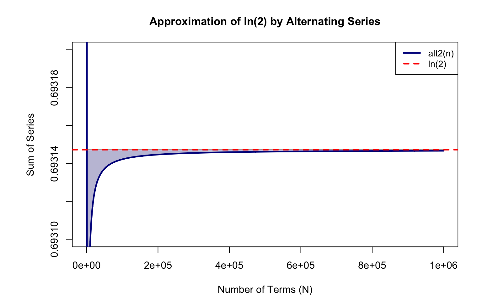

Key insight: The series converges slowly, requiring about 1 million terms to get within 0.0000005 of ln(2). Computing this in pure R would be much slower.

5. Example 2: Kernel Density Estimation

Problem

Compute kernel density estimates for earthquake magnitude data using a Gaussian kernel.

Why C? With n=223 data points and m=100 grid points, we perform 22,300 kernel evaluations. For larger datasets (n=10,000, m=500), that’s 5 million calculations.

Loading the Data

library(ggplot2)

# Load earthquake data
data <- read.table(file = "SearchResults.txt", sep = "", skip = 2, fill = T)
colnames(data) <- c("DATE", "TIME", "ET", "GT", "MAG", "M", "LAT", 
                    "LON", "DEPTH", "Q", "EVID", "NPH", "NGRM")

magnitudes <- data$MAG
cat("Number of earthquakes:", length(magnitudes), "\n")

Number of earthquakes: 219

cat("Magnitude range:", sprintf("[%.2f, %.2f]", min(magnitudes), max(magnitudes)), "\n")

Magnitude range: [4.00, 6.70]

C Implementation

Rcpp::cppFunction("
NumericVector kernel_density(NumericVector g, NumericVector x, double h) {
  int m = g.size();  // number of grid points
  int n = x.size();  // number of data points
  NumericVector y(m);  // output density estimates
  
  double sqrt_2pi = sqrt(2.0 * M_PI);
  
  // For each grid point
  for(int i = 0; i < m; ++i) {
    y[i] = 0.0;
    // Sum contributions from all data points
    for(int j = 0; j < n; ++j) {
      double z = (g[i] - x[j]) / h;
      y[i] += exp(-0.5 * z * z) / (h * sqrt_2pi);
    }
    y[i] /= n;  // Normalize
  }
  
  return y;
}
")

C++ features used:

NumericVector: Rcpp’s vector type that interfaces with R
.size(): Method to get vector length
Nested loops: The inner loop runs n times for each of m iterations
Mathematical functions: sqrt(), exp(), pow()

Computing and Plotting

# Calculate bandwidth using Scott's rule
h <- bw.nrd(magnitudes)
cat("Bandwidth (Scott's rule):", sprintf("%.4f", h), "\n")

Bandwidth (Scott's rule): 0.1319

# Create grid
g <- seq(min(magnitudes), max(magnitudes), length = 100)

# Call C function
y <- kernel_density(g, magnitudes, h)

# Create plot
kde_data <- data.frame(Magnitude = g, Density = y)

par(mar = c(4.5, 4.5, 3.5, 2))
plot(kde_data$Magnitude, kde_data$Density,
     type = "l", col = "darkblue", lwd = 2.5,
     xlab = "Magnitude (m)", ylab = "Density f(m)",
     main = "Kernel Density Estimate of Earthquake Magnitudes",
     cex.lab = 1.0, cex.main = 1.1,
     ylim = c(0, max(kde_data$Density) * 1.1))

rug(magnitudes, col = "red", lwd = 0.8, ticksize = 0.03)

legend("topright",
       legend = c("Kernel Density", "Data Points"),
       col = c("darkblue", "red"),
       lty = c(1, NA),
       pch = c(NA, 124),
       lwd = c(2.5, 1),
       bg = "white",
       cex = 0.9)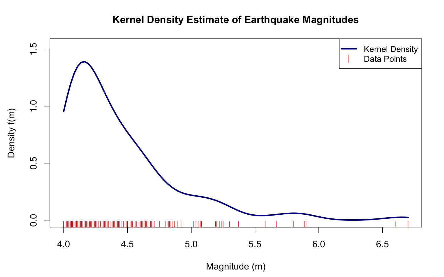

Performance Comparison

# R version for comparison
kernel_density_r <- function(g, x, h) {
  m <- length(g)
  n <- length(x)
  y <- numeric(m)
  sqrt_2pi <- sqrt(2 * pi)
  
  for(i in 1:m) {
    for(j in 1:n) {
      z <- (g[i] - x[j]) / h
      y[i] <- y[i] + exp(-0.5 * z^2) / (h * sqrt_2pi)
    }
    y[i] <- y[i] / n
  }
  return(y)
}

# Benchmark
cat("\nPerformance comparison:\n")


Performance comparison:

system.time(y_r <- kernel_density_r(g, magnitudes, h))

   user  system elapsed 
  0.005   0.000   0.005

system.time(y_cpp <- kernel_density(g, magnitudes, h))

   user  system elapsed 
  0.001   0.000   0.001

6. Example 3: Numerical Integration

Problem

Approximate the integral of a shifted Pareto density:

\[f(x) = (p-1)c^{p-1}(x+c)^{-p}, \quad x \geq 0\]

Using the trapezoidal rule with 1 million grid points.

Implementation

Rcpp::cppFunction("
double paretoint(double xmax, double c, double p) {
  int n = 1000000;  // 1 million grid points
  double dx = xmax / (n - 1);
  double integral = 0.0;
  
  // Coefficient: (p-1) * c^(p-1)
  double coef = (p - 1) * pow(c, p - 1);
  
  // Trapezoidal rule
  double f0 = coef * pow(c, -p);
  double fn = coef * pow(xmax + c, -p);
  
  double sum_middle = 0.0;
  for(int i = 1; i < n - 1; ++i) {
    double x = i * dx;
    double fx = coef * pow(x + c, -p);
    sum_middle += fx;
  }
  
  integral = dx * (0.5 * f0 + sum_middle + 0.5 * fn);
  return integral;
}
")

Case 1: c = 3, p = 2

c1 <- 3
p1 <- 2

xmax_values1 <- c(10, 25, 50, 75, 100, 150, 200, 300, 400, 500, 
                  600, 700, 800, 900, 1000)

integral_values1 <- sapply(xmax_values1, function(xm) {
  paretoint(xm, c1, p1)
})

df1 <- data.frame(xmax = xmax_values1, integral = integral_values1)

par(mar = c(4.5, 4.5, 3.5, 2))
plot(df1$xmax, df1$integral,
     type = "b", col = "darkblue", lwd = 2.5, pch = 19, cex = 1.2,
     xlab = "xmax", ylab = "paretoint(xmax, 3, 2)",
     main = "Pareto Integral: c = 3, p = 2",
     las = 1, cex.lab = 1.1, cex.main = 1.2,
     panel.first = grid(col = "gray90", lty = "solid", lwd = 0.5))
abline(h = 1, col = "red", lwd = 2, lty = 2)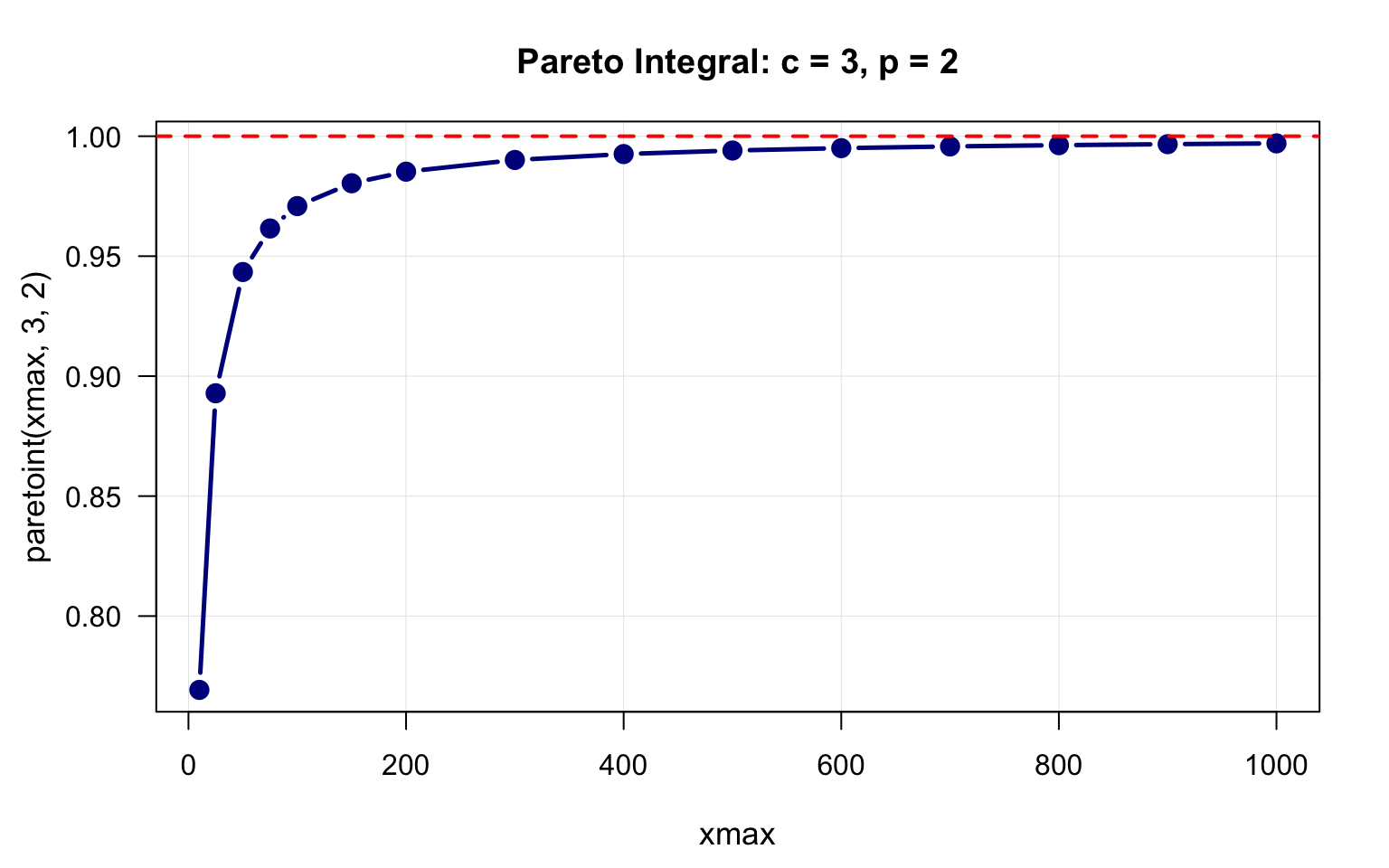

Case 2: c = 12, p = 3.5

c2 <- 12
p2 <- 3.5

xmax_values2 <- c(10, 25, 50, 75, 100, 150, 200, 300, 400, 500, 
                  600, 700, 800, 900, 1000)

integral_values2 <- sapply(xmax_values2, function(xm) {
  paretoint(xm, c2, p2)
})

df2 <- data.frame(xmax = xmax_values2, integral = integral_values2)

par(mar = c(4.5, 4.5, 3.5, 2))
plot(df2$xmax, df2$integral,
     type = "b", col = "darkgreen", lwd = 2.5, pch = 19, cex = 1.2,
     xlab = "xmax", ylab = "paretoint(xmax, 12, 3.5)",
     main = "Pareto Integral: c = 12, p = 3.5",
     las = 1, cex.lab = 1.1, cex.main = 1.2,
     ylim = c(0, max(df2$integral) * 1.1),
     panel.first = grid(col = "gray90", lty = "solid", lwd = 0.5))
abline(h = 1, col = "red", lwd = 2, lty = 2)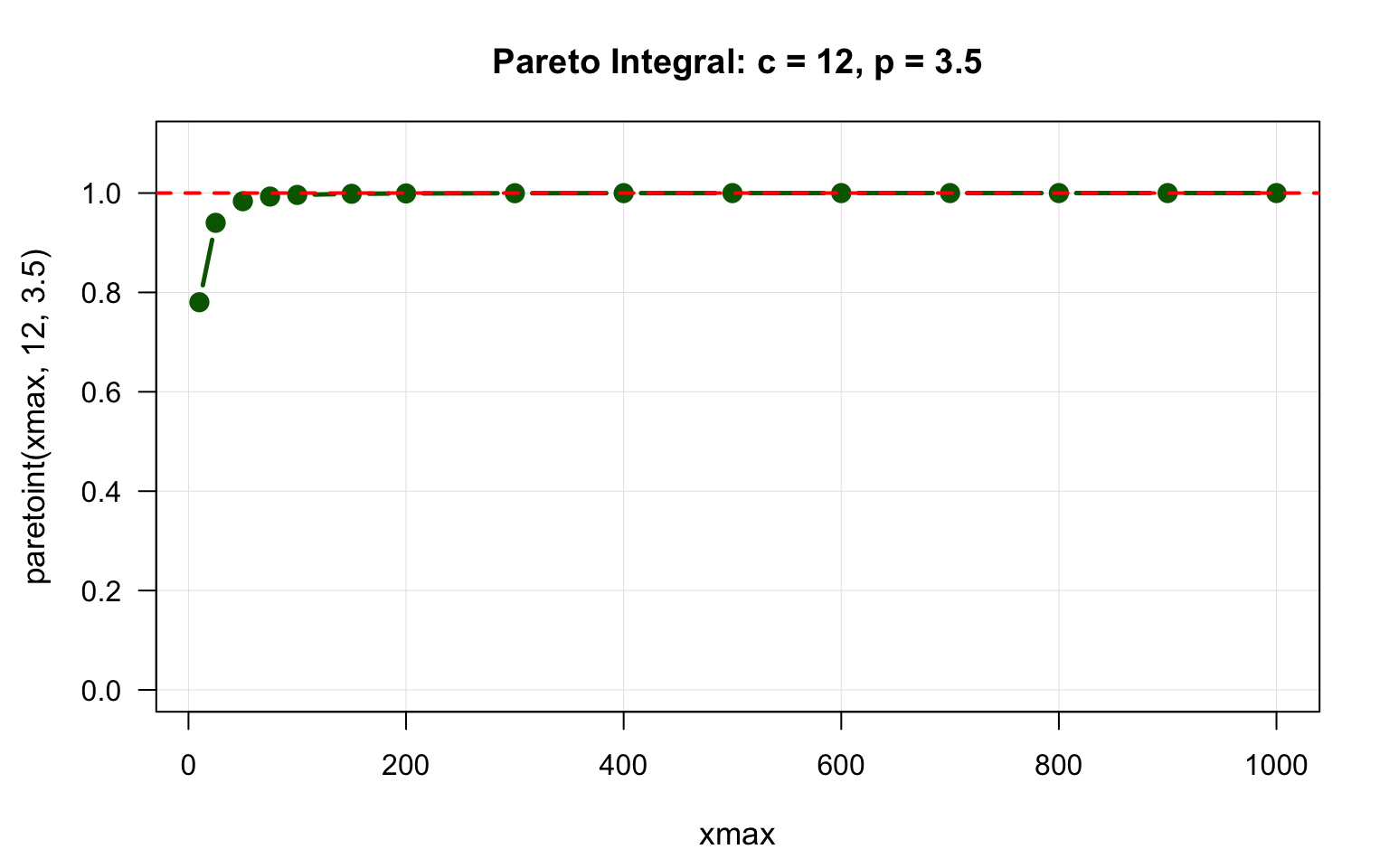

Interpretation: Both integrals converge to 1 (shown by red dashed line), which is expected since we’re integrating a probability density function. The convergence is faster for larger c and p values.

7. Example 4: Nadaraya-Watson Kernel Regression with Bootstrap Confidence Intervals

This example demonstrates a more advanced application combining C functions with statistical inference. We’ll implement kernel regression to analyze the relationship between petroleum taxes and consumption, then use bootstrap methods to quantify uncertainty.

Problem

Given data on petroleum taxes (X) and consumption (Y), we want to:

Estimate the relationship using Nadaraya-Watson kernel regression
Compute bootstrap confidence intervals for the regression curve
Visualize the results with uncertainty bands

C Implementation: Nadaraya-Watson Estimator

The Nadaraya-Watson estimator computes a weighted average of Y values at each grid point g:

\[\hat{f}(g) = \frac{\sum_{i=1}^{n} K\left(\frac{g - X_i}{b}\right) Y_i}{\sum_{i=1}^{n} K\left(\frac{g - X_i}{b}\right)}\]

where K is the Gaussian kernel and b is the bandwidth.

Rcpp::cppFunction("
NumericVector nadaraya_watson(int n, NumericVector X, NumericVector Y, 
                               int m, NumericVector g2, double b) {
  NumericVector res2(m);
  
  // Compute kernel regression estimates at each grid point
  for(int j = 0; j < m; j++) {
    double numerator = 0.0;
    double denominator = 0.0;
    
    // Sum over all observations
    for(int i = 0; i < n; i++) {
      // Gaussian kernel: exp(-0.5 * ((x - xi) / b)^2)
      double u = (g2[j] - X[i]) / b;
      double kernel_weight = exp(-0.5 * u * u);
      
      numerator += kernel_weight * Y[i];
      denominator += kernel_weight;
    }
    
    // Compute the weighted average
    if(denominator > 0) {
      res2[j] = numerator / denominator;
    } else {
      res2[j] = NA_REAL;
    }
  }
  
  return res2;
}
")

Key implementation details:

Nested loops: The outer loop iterates over m grid points, the inner over n observations
Gaussian kernel: We use \(K(u) = \exp(-0.5u^2)\) without the normalizing constant (it cancels in the ratio)
Numerical stability: Check for denominator > 0 before division
NA handling: Return NA_REAL for grid points with no nearby data

Loading the Data

We’ll use petroleum tax and consumption data to illustrate the method:

# Petroleum taxes and consumption data
url <- "https://people.sc.fsu.edu/~jburkardt/datasets/regression/x15.txt"
data_raw <- readLines(url)
data_lines <- data_raw[grep("^\\s*[0-9]", data_raw)]
data_lines <- data_lines[-(1:2)]
data <- read.table(text = data_lines)

X <- data$V2  # Petroleum tax
Y <- data$V6  # Petroleum consumption

cat("Sample size:", length(X), "\n")

Sample size: 48

cat("Tax range: [", min(X), ",", max(X), "]\n")

Tax range: [ 5 , 10 ]

cat("Consumption range: [", min(Y), ",", max(Y), "]\n")

Consumption range: [ 344 , 968 ]

Computing the Kernel Regression Estimate

n <- length(X)
b <- bw.nrd(X)  # Scott's bandwidth rule
m <- 100
g2 <- seq(min(X), max(X), length.out = m)

# Compute kernel regression estimates
kernel_fit <- nadaraya_watson(n, X, Y, m, g2, b)

# Initial plot
par(mar = c(4.5, 4.5, 3.5, 2))
plot(X, Y, pch = 19, col = "gray50", cex = 0.8,
     xlab = "Petroleum Tax", ylab = "Consumption",
     main = "Kernel Regression: Tax vs. Consumption")
lines(g2, kernel_fit, col = "blue", lwd = 2.5)
legend("topright", legend = "Kernel Estimate", 
       col = "blue", lwd = 2.5, bg = "white")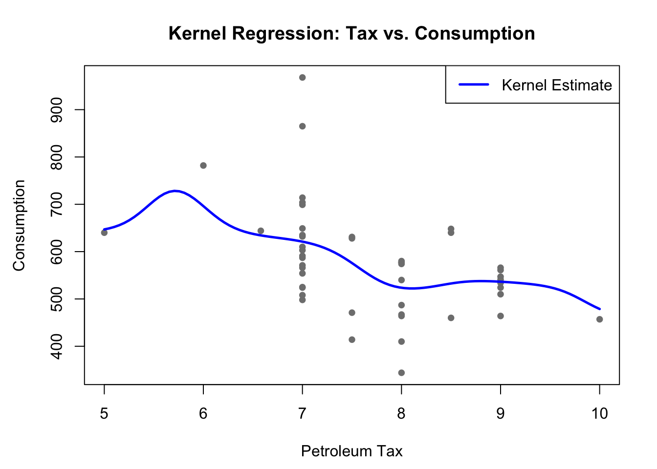

Bootstrap Confidence Intervals

To quantify uncertainty in our estimates, we use the bootstrap:

Resample: Draw n pairs \((X_i, Y_i)\) with replacement from the original data
Refit: Compute kernel regression on the bootstrap sample
Repeat: Do this B = 200 times
Quantiles: At each grid point, compute the 2.5th and 97.5th percentiles

B <- 200  # Number of bootstrap samples
boot_mat <- matrix(NA, nrow = B, ncol = m)

# Bootstrap loop
for(i in 1:B) {
  # Resample with replacement
  idx <- sample(1:n, n, replace = TRUE)
  X_boot <- X[idx]
  Y_boot <- Y[idx]
  
  # Compute kernel regression on bootstrap sample
  boot_mat[i, ] <- nadaraya_watson(n, X_boot, Y_boot, m, g2, b)
}

# Compute confidence bounds
lower_ci <- apply(boot_mat, 2, quantile, probs = 0.025, na.rm = TRUE)
upper_ci <- apply(boot_mat, 2, quantile, probs = 0.975, na.rm = TRUE)

Why bootstrap works here:

Kernel regression is a smooth function of the data
Bootstrap resampling preserves the joint distribution of (X, Y)
Percentile method provides valid confidence bands under mild conditions
The 200 bootstrap samples give stable percentile estimates

Final Visualization

par(mar = c(4.5, 4.5, 3.5, 2))
plot(X, Y, pch = 19, col = "gray50", cex = 0.8, main = "Kernel Regression with 95% Bootstrap CI",
     xlab = "Petroleum Tax", ylab = "Consumption", cex.lab = 1.1, cex.main = 1.2)
lines(g2, kernel_fit, col = "blue", lwd = 2.5)
polygon(c(g2, rev(g2)), c(lower_ci, rev(upper_ci)), col = rgb(1, 0, 0, 0.2), border = NA)

lines(g2, lower_ci, col = "red", lty = 2, lwd = 1.5)
lines(g2, upper_ci, col = "red", lty = 2, lwd = 1.5)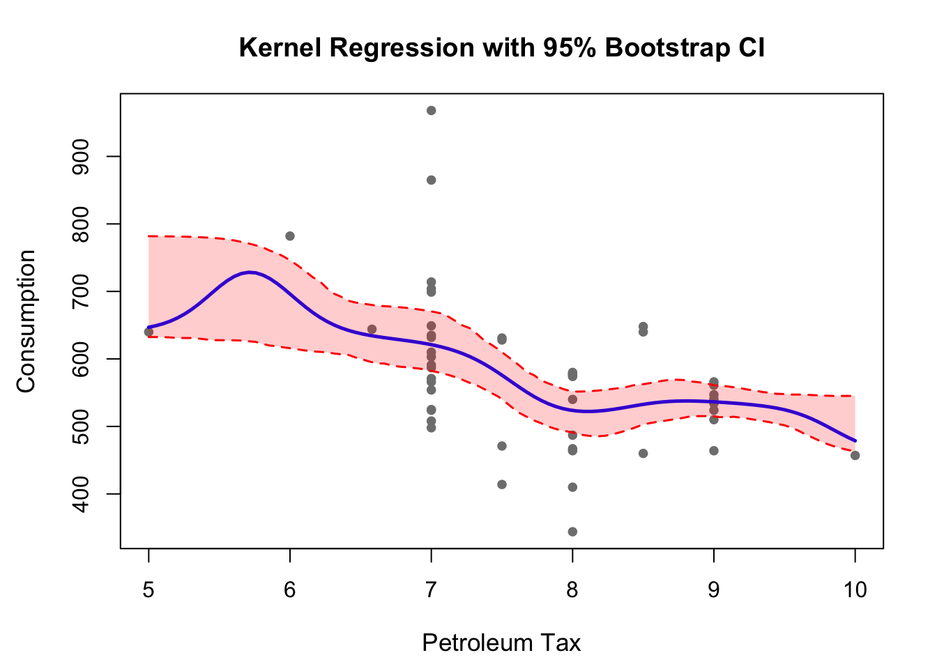

8. Common Pitfalls

Array Indexing

// C++ uses 0-based indexing
for(int i = 0; i < n; ++i) {  // 0 to n-1
  x[i] = ...
}

// R uses 1-based indexing
for(i in 1:n) {  // 1 to n
  x[i] <- ...
}

Integer Division

double result = 5 / 2;      // Result: 2.0 (integer division)
double result = 5.0 / 2.0;  // Result: 2.5 (correct)

Power Functions

pow(-1, i)    // Correct
(-1)^i        // WRONG. ^ is XOR in C++, not exponentiation

1. Introduction

2. Why Call C from R?

Performance Comparison

When to Use C from R

3. Getting Started with Rcpp

Installation

Your First C Function in R

4. Example 1: Alternating Series Convergence

Problem

Implementation

Visualization

5. Example 2: Kernel Density Estimation

Problem

Loading the Data

C Implementation

Computing and Plotting

Performance Comparison

6. Example 3: Numerical Integration

Problem

Implementation

Case 1: c = 3, p = 2

Case 2: c = 12, p = 3.5

7. Example 4: Nadaraya-Watson Kernel Regression with Bootstrap Confidence Intervals

Problem

C Implementation: Nadaraya-Watson Estimator

Loading the Data

Computing the Kernel Regression Estimate

Bootstrap Confidence Intervals

Final Visualization

8. Common Pitfalls

Array Indexing

Integer Division

Power Functions

Further Reading