In previous posts, we’ve explored the Potential Outcomes framework and matching methods for causal inference. Today, we’ll dive deeper into propensity score methods, which offer a powerful and flexible approach to addressing selection bias in observational studies.
1. Introduction
The propensity score is defined as:
\[p(X_i) = P(D_i = 1 | X_i)\] Where:
\(D_i\) is the treatment indicator (1 if treated, 0 if control)
\(X_i\) is a vector of observed covariates for unit \(i\)
If we have two districts with the same propensity score, they have the same probability of receiving treatment based on their observed characteristics. This means that among districts with similar propensity scores, treatment assignment is assuming random - aiming to achieve a quasi-experimental design.
A property of propensity scores is that if treatment assignment is strongly ignorable given \(X\), then:
This means that conditioning on the propensity score is sufficient to achieve independence between potential outcomes and treatment assignment. In other words, within strata of units with similar propensity scores, the distribution of covariates should be similar between treated and control groups.
1.1 Propensity Score Methods
There are three main ways to use propensity scores:
Matching: Pair treated and control units with similar propensity scores
Inverse Probability of Treatment Weighting (IPTW): Weight observations by the inverse of their probability of receiving their observed treatment
Stratification: Divide the sample into strata based on propensity score ranges
In this post, we’ll focus on IPTW, with a practical example using educational data.
2. Inverse Probability of Treatment Weighting (IPTW)
2.1 Mathematical Foundation
IPTW is based on creating a pseudo-population where treatment assignment is independent of confounders. The key insight is that by weighting each observation by the inverse of its probability of receiving the treatment it actually received, we can balance the covariate distributions between treatment groups.
For the Average Treatment Effect (ATE), the weights are:
For treated units (\(D_i = 1\)): \(w_i = \frac{1-p(X_i)}{p(X_i)}\)
For control units (\(D_i = 0\)): \(w_i = 1\)
Intuition Behind IPTW
The weights create a pseudo-population where:
Treated units who were unlikely to be treated (low \(p(X_i)\)) get high weights
Control units who were likely to be treated (high \(p(X_i)\)) get high weights
This “fills in” the missing counterfactuals by upweighting similar units from the opposite group
3. HSLS:09 Science Museum Practical Example
Leveraging the High School Longitudinal Study (HSLS:09), this example aims to answer the following questions:
Treament: What individual and contextual factors are associated with students’ likelihood of visiting science museums or planetariums during high school?
Science Identity Formation: Does participation in informal science learning experiences—such as visiting a science museum or planetarium between 9th and 11th grade—positively influence the development of a science identity?
STEM Major Intentions: Does exposure to science museums or planetariums during high school increase the likelihood of pursuing a STEM major in college?
Note
The analysis data file include 6,481 9th grade students with observed treatment group status and no-zero value of sample weight (W3W1W2STU).Missing rate range from 1% to 19%. Dealing with missing values using likewise deletion is problematic, given the sample size will be reduced considerably and will introduce bias unless the data is missing completely at random (Enders, 2010). In this study we impute single values using stochastic imputations and chained equations embedded in mice r package.
The final analysis data file includes 8,106 college-bound students and the following variables:
Treatment indicator:
- p2museum = visited a science-related museum/planetarium between 9th and 11th grade (1 = Yes, 0 = No) Dependent variables (DVs):
- x2sciid = 11th-grade science identity scale (standardized z-score)
- collegeSTEMmajorasp = binary indicator of whether the student aspired to or declared a STEM major while enrolled in college (1 = Yes, 0 = No) Pre-treatment covariates:
- x1sciid = 9th-grade baseline science identity scale (standardized z-score)
- stemoccasp9th = binary indicator of whether the student aspired to a STEM occupation in 9th grade School-level covariates (baseline, 9th grade):
- x1locale = school locale: City, Suburb, Town, Rural (ref)
- x1control = school control: Public, Catholic or other Private School (ref)
- x1region = U.S. census region of the school: Northeast (ref), Midwest, South, West
- a1mspdintrst = binary indicator for whether the school sponsored a math or science after-school program (Yes/No)
- a1msmentor = binary indicator for whether the school paired students with mentors in math or science (Yes/No) Student-level IVs: background characteristics:
- x1race = White (ref), Asian, Black, Latino, Multiracial, Native American, Other
- x1sex = binary sex indicator (0 = Male, 1 = Female)
- x1sesq5 = socioeconomic status quintile, First quintile (ref, lowest), Second, Third, Fourth, and Fifth quintile (highest)
- x1txmscr = 9th-grade math achievement score (IRT-scaled)
- x1sciint = science course interest scale (standardized z-score)
- x1stuedexpct = student’s highest educational expectation, categorized as Uncertain (ref), High School, Bachelor’s, Master’s, or PhD
- x1schoolbel = 9th-grade student-perceived school belonging scale (standardized z-score) Student-leve IVs: formal and informal STEM experiences (9th grade):
- s1alg1m09 = binary indicator of whether the student took Algebra I in 9th grade (Yes/No)
- s1sfall09 = binary indicator of whether the student took a science course in fall 2009 (Yes/No)
- p1campms = binary indicator of whether the student participated in math or science camp outside of school in last year (Yes/No)
- p1fixed = binary indicator of whether parents built or fixed something with 9th grader in last year (Yes/No)
- p1sciproj = binary indicator of whether the helped 9th grader with a school science fair project in last year with 9th grader in last year (Yes/No)
Analysis the outcome, ATE, ATT, ATU:
Used doubly robust approach
Consider using MLM random slop (two levels: student level and school level)
Then conduct robustness check, use sensemakr to run the sensitivity analysis
Use student’s 9th grade science identity as benchmark covariates
Code
rm(list =ls())library(tidyverse)library(skimr)library(flextable)library(table1)library(tableone)library(knitr)library(MatchIt)library(WeightIt)library(cobalt) #for love plots library(marginaleffects)library(sensemakr) #sensitivity analysislibrary(patchwork)library(car)library(naniar)library(mice)library(haven)library(lm.beta) #standardized beta coef (for comparing effect sizes)library(lme4) #for fixed modelslibrary(survey) #for weights and robust SEslibrary(broom) #convert model into tidy data frameslibrary(lme4)library(merTools)library(lmerTest)library(WeMix) data <-readRDS("hslspsm_imputed.rds")
3.1 Descriptive Analysis
Code
length(unique(data$STU_ID))
[1] 6481
Code
length(unique(data$SCH_ID))
[1] 933
Code
autofit(as_flextable(table(data$p2museum)))
Var1
Count
Percent
Control
3,805
58.7%
Treatment
2,676
41.3%
Total
6,481
100.0%
Code
#combine Native American and Other other all into others categories due to small subpopulationdata <- data %>%mutate(x1race =fct_collapse(x1race,Other =c("Native American", "Other") # <- names to merge ))#Descriptive Analysisdescr1 <-table1(~ x1sciid + stemoccasp9th +#pre-IVs x1locale + x1control + x1region + a1mspdintrst + a1msmentor +#school-level IV x1race + x1sex + x1sesq5 + x1schoolbel + x1txmscr + x1sciint + x1stuedexpct +#student-level IV background s1alg1m09 + s1sfall09 + p1campms + p1fixed + p1sciproj + x2sciid + collegeSTEMmajorasp |as.factor(p2museum), data = data)descr1
Control (N=3805)
Treatment (N=2676)
Overall (N=6481)
x1sciid
Mean (SD)
0.0450 (0.998)
0.214 (1.01)
0.115 (1.01)
Median [Min, Max]
-0.300 [-2.25, 2.15]
0.270 [-2.89, 2.27]
0.270 [-2.89, 2.27]
stemoccasp9th
non-STEM
2558 (67.2%)
1705 (63.7%)
4263 (65.8%)
STEM
1247 (32.8%)
971 (36.3%)
2218 (34.2%)
x1locale
Rural
924 (24.3%)
553 (20.7%)
1477 (22.8%)
City
1100 (28.9%)
841 (31.4%)
1941 (29.9%)
Suburb
1330 (35.0%)
996 (37.2%)
2326 (35.9%)
Town
451 (11.9%)
286 (10.7%)
737 (11.4%)
x1control
Catholic or other private
664 (17.5%)
600 (22.4%)
1264 (19.5%)
Public
3141 (82.5%)
2076 (77.6%)
5217 (80.5%)
x1region
Northeast
604 (15.9%)
416 (15.5%)
1020 (15.7%)
Midwest
948 (24.9%)
757 (28.3%)
1705 (26.3%)
South
1579 (41.5%)
1029 (38.5%)
2608 (40.2%)
West
674 (17.7%)
474 (17.7%)
1148 (17.7%)
a1mspdintrst
No
1815 (47.7%)
1258 (47.0%)
3073 (47.4%)
Yes
1990 (52.3%)
1418 (53.0%)
3408 (52.6%)
a1msmentor
No
2521 (66.3%)
1694 (63.3%)
4215 (65.0%)
Yes
1284 (33.7%)
982 (36.7%)
2266 (35.0%)
x1race
White
2062 (54.2%)
1546 (57.8%)
3608 (55.7%)
Asian
302 (7.9%)
205 (7.7%)
507 (7.8%)
Black
469 (12.3%)
245 (9.2%)
714 (11.0%)
Latino
589 (15.5%)
403 (15.1%)
992 (15.3%)
Multiracial
335 (8.8%)
250 (9.3%)
585 (9.0%)
Other
48 (1.3%)
27 (1.0%)
75 (1.2%)
x1sex
Male
2005 (52.7%)
1221 (45.6%)
3226 (49.8%)
Female
1800 (47.3%)
1455 (54.4%)
3255 (50.2%)
x1sesq5
First quintile (lowest)
662 (17.4%)
274 (10.2%)
936 (14.4%)
Second quintile
691 (18.2%)
342 (12.8%)
1033 (15.9%)
Third quintile
739 (19.4%)
459 (17.2%)
1198 (18.5%)
Fourth quintile
748 (19.7%)
579 (21.6%)
1327 (20.5%)
Fifth quintile (highest)
965 (25.4%)
1022 (38.2%)
1987 (30.7%)
x1schoolbel
Mean (SD)
0.118 (0.982)
0.206 (0.956)
0.155 (0.972)
Median [Min, Max]
0.0100 [-3.87, 2.88]
0.180 [-3.87, 2.64]
0.100 [-3.87, 2.88]
x1txmscr
Mean (SD)
41.2 (11.9)
43.0 (11.7)
41.9 (11.9)
Median [Min, Max]
41.3 [15.8, 69.9]
43.0 [13.6, 69.9]
42.1 [13.6, 69.9]
x1sciint
Mean (SD)
0.0291 (0.981)
0.123 (0.998)
0.0681 (0.989)
Median [Min, Max]
0.160 [-3.15, 3.05]
0.160 [-2.59, 3.46]
0.160 [-3.15, 3.46]
x1stuedexpct
Uncertain
795 (20.9%)
488 (18.2%)
1283 (19.8%)
High school
453 (11.9%)
217 (8.1%)
670 (10.3%)
Bachelor
922 (24.2%)
613 (22.9%)
1535 (23.7%)
Master
817 (21.5%)
639 (23.9%)
1456 (22.5%)
PhD
818 (21.5%)
719 (26.9%)
1537 (23.7%)
s1alg1m09
No
1653 (43.4%)
1267 (47.3%)
2920 (45.1%)
Yes
2152 (56.6%)
1409 (52.7%)
3561 (54.9%)
s1sfall09
No
629 (16.5%)
355 (13.3%)
984 (15.2%)
Yes
3176 (83.5%)
2321 (86.7%)
5497 (84.8%)
p1campms
No
3693 (97.1%)
2529 (94.5%)
6222 (96.0%)
Yes
112 (2.9%)
147 (5.5%)
259 (4.0%)
p1fixed
No
2180 (57.3%)
1385 (51.8%)
3565 (55.0%)
Yes
1625 (42.7%)
1291 (48.2%)
2916 (45.0%)
p1sciproj
No
2397 (63.0%)
1562 (58.4%)
3959 (61.1%)
Yes
1408 (37.0%)
1114 (41.6%)
2522 (38.9%)
x2sciid
Mean (SD)
0.0465 (0.995)
0.189 (1.00)
0.105 (1.00)
Median [Min, Max]
0.0400 [-2.15, 2.54]
0.0800 [-2.83, 2.10]
0.0400 [-2.83, 2.54]
collegeSTEMmajorasp
No
3029 (79.6%)
2034 (76.0%)
5063 (78.1%)
Yes
776 (20.4%)
642 (24.0%)
1418 (21.9%)
Compute the navie effect without adding PS and Weighting
Unconditional Navie Estimate (No PS, no sample weight, single level without covaraite adjustment)
Code
m00 <-lm(x2sciid ~ p2museum, data = data)summary(m00)
Call:
lm(formula = x2sciid ~ p2museum, data = data)

Residuals:
     Min       1Q   Median       3Q      Max
-3.01610 -0.58651 -0.00651  0.61349  2.49201

Coefficients:
                  Estimate Std. Error t value Pr(>|t|)
(Intercept)        0.04651    0.01617   2.875  0.00405 **
p2museumTreatment  0.14217    0.02517   5.648 1.69e-08 ***
---
Signif. codes:  0 '***' 0.001 '**' 0.01 '*' 0.05 '.' 0.1 ' ' 1

Residual standard error: 0.9977 on 6479 degrees of freedom
Multiple R-squared:  0.004899,  Adjusted R-squared:  0.004746
F-statistic:  31.9 on 1 and 6479 DF,  p-value: 1.694e-08
Code
sqrt(hccm(m00)[2,2])
[1] 0.0252022
Code
m000 <-glm(collegeSTEMmajorasp ~ p2museum, data = data, family ="binomial" )summary(m000)
Call:
glm(formula = collegeSTEMmajorasp ~ p2museum, family = "binomial",
    data = data)

Coefficients:
                  Estimate Std. Error z value Pr(>|z|)
(Intercept)       -1.36184    0.04023 -33.848  < 2e-16 ***
p2museumTreatment  0.20866    0.06056   3.445  0.00057 ***
---
Signif. codes:  0 '***' 0.001 '**' 0.01 '*' 0.05 '.' 0.1 ' ' 1

(Dispersion parameter for binomial family taken to be 1)

    Null deviance: 6809.9  on 6480  degrees of freedom
Residual deviance: 6798.1  on 6479  degrees of freedom
AIC: 6802.1

Number of Fisher Scoring iterations: 4
Navie Estimate (No PS, no sample weight, single level with covaraite adjustment)
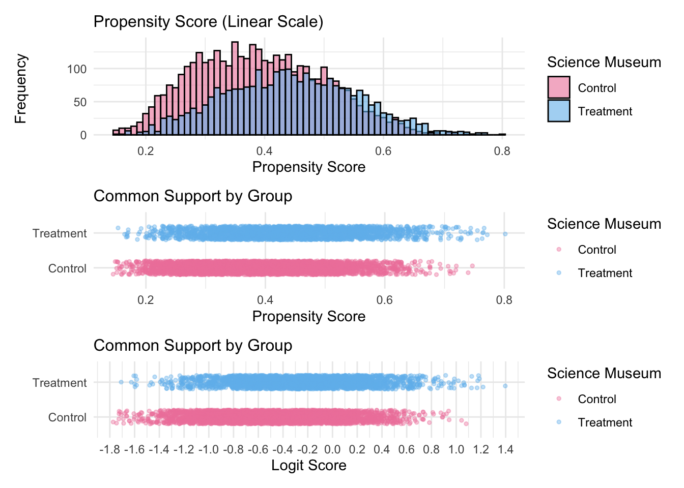
data_trimmed <- data %>%filter(pscorelogodd >=-1.6& pscorelogodd <=1.0)table(data_trimmed$p2museum)
  Control Treatment
     3783      2660
Code
#total loss 41 cases
3.3 IPTW, balance with IPTW*W3W1W2STU
Compare two weight methods:
First, use non-weighted PSM, them multiply by the ate/att/atc, we get: w.ate_W3W1W2STU; w.att_W3W1W2STU; w.atc_W3W1W2STU
Second, use sample weight in the propensity score stage, then compute final weights as the product of the sampling weight and the propensity score weight: w.ate.w_W3W1W2STU; w.att.w_W3W1W2STU; w.atc.w_W3W1W2STU.
Combined weight with non-weighted PSM
Code
#normalize the panel weightdata_trimmed <- data_trimmed %>%mutate(W3W1W2STU_norm = W3W1W2STU /mean(W3W1W2STU, na.rm =TRUE))#calculate IPTW (ATE, ATT, ATU)data_trimmed <- data_trimmed %>%#weight based on the treatmentmutate(D =ifelse(p2museum =="Treatment", 1, 0),w.ate = (D * (1/pscore)) + ((1- D) * (1/(1- pscore))),w.att = (D) + ((1- D) * (pscore/(1- pscore))),w.atc = (D * ((1- pscore)/pscore)) + (1- D),#balance the weight based on the control levelw.ate_W3W1W2STU = w.ate*W3W1W2STU_norm,w.att_W3W1W2STU = w.att*W3W1W2STU_norm,w.atc_W3W1W2STU = w.atc*W3W1W2STU_norm )table(data_trimmed$D)
   0    1
3783 2660
Code
table(data_trimmed$p2museum)
  Control Treatment
     3783      2660
Check the data balance
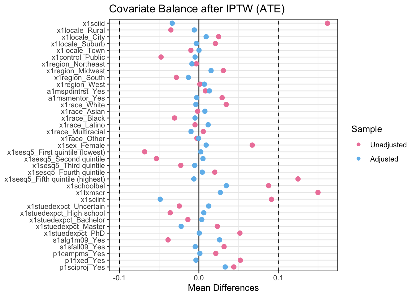
SMD is <0.10 for all covariates
Code
#question? check the balance only for w.ate or for w.ate_W3W1W2STUcovars <-c("x1sciid", "x1locale", "x1control", "x1region", "a1mspdintrst", "a1msmentor","x1race", "x1sex", "x1sesq5", "x1schoolbel", "x1txmscr", "x1sciint", "x1stuedexpct", "s1alg1m09", "s1sfall09","p1campms", "p1fixed", "p1sciproj") bal_ate <-bal.tab(x = data_trimmed[, covars],treat = data_trimmed$D,weights = data_trimmed$w.ate_W3W1W2STU,estimand ="ATE",s.d.denom ="pooled", # std-diff denominatorm.threshold = .1, # ±0.10 rule of thumbun =TRUE)bal_ate
#questions? what's the Effective sample sizes mean here?#The effective numbers after applying the IPTW*W3W1W2STU weights had a sample of about 1,574 controls and 959 treated cases.love.plot(bal_ate,stats ="mean.diffs",abs =FALSE, binary ="std", thresholds =c(m = .10),colors =c("#ee84a8", "#71bced"),title ="Covariate Balance after IPTW (ATE)") +theme_bw()
Get the descriptive stats after weighting (ATE)
Code
#create survey design object using IPTW weightsdesign <-svydesign(ids =~1, weights =~w.ate_W3W1W2STU, data = data_trimmed)#create post-weighting descriptive table by treatment grouptable_weighted <-svyCreateTableOne(vars = covars, strata ="p2museum", data = design)print(table_weighted)
#estimate navie ATE of museum on sciidate_sciid <-lm(x2sciid ~ x1sciid +#pre-IVs p2museum, data = data_trimmed, weights = w.ate_W3W1W2STU)sqrt(hccm(ate_sciid)[3,3])
[1] 0.03523017
Code
table.ate_sciid <-tidy.coeftable(ate_sciid) knitr::kable(table.ate_sciid, digits =3, caption ="nested1 ATE weighted results of linear regression on science identity")
nested1 ATE weighted results of linear regression on science identity
table.ate_sciid2 <-tidy.coeftable(ate_sciid2)knitr::kable(table.ate_sciid2, digits =3, caption ="nested 2 ATE weighted results of linear regression on science identity")
nested 2 ATE weighted results of linear regression on science identity
Variable
Coefficient
SE
Beta
p_value
Sig
(Intercept)
-0.221
0.077
NA
0.004
**
x1sciid
0.369
0.013
0.374
0.000
***
p2museumTreatment
0.058
0.022
0.029
0.008
**
x1localeCity
-0.042
0.032
-0.020
0.191
x1localeSuburb
-0.066
0.031
-0.032
0.031
*
x1localeTown
-0.112
0.040
-0.036
0.005
**
x1controlPublic
0.053
0.044
0.014
0.224
x1regionMidwest
0.010
0.036
0.004
0.784
x1regionSouth
0.007
0.033
0.003
0.840
x1regionWest
0.002
0.036
0.001
0.958
a1mspdintrstYes
-0.003
0.022
-0.001
0.910
a1msmentorYes
-0.005
0.023
-0.002
0.825
x1raceAsian
0.138
0.060
0.026
0.021
*
x1raceBlack
0.005
0.036
0.002
0.890
x1raceLatino
-0.119
0.032
-0.052
0.000
***
x1raceMultiracial
-0.052
0.042
-0.015
0.211
x1raceOther
0.208
0.098
0.024
0.034
*
x1sexFemale
-0.120
0.022
-0.061
0.000
***
x1sesq5Second quintile
-0.020
0.035
-0.008
0.579
x1sesq5Third quintile
0.014
0.036
0.006
0.695
x1sesq5Fourth quintile
-0.001
0.038
0.000
0.974
x1sesq5Fifth quintile (highest)
0.072
0.039
0.030
0.067
.
x1schoolbel
-0.023
0.012
-0.023
0.059
.
x1txmscr
0.006
0.001
0.068
0.000
***
x1sciint
0.076
0.013
0.076
0.000
***
x1stuedexpctHigh school
0.069
0.039
0.023
0.080
.
x1stuedexpctBachelor
0.026
0.033
0.011
0.438
x1stuedexpctMaster
0.082
0.034
0.034
0.016
*
x1stuedexpctPhD
0.194
0.035
0.081
0.000
***
Result with IPW science identity
Code
#estimate ATE of museum on sciidate_dr_sciid <-lm(x2sciid ~ x1sciid +#pre-IVs p2museum + x1locale + x1control + x1region + a1mspdintrst + a1msmentor +#school-level IV x1race + x1sex + x1sesq5 + x1schoolbel + x1txmscr + x1sciint + x1stuedexpct +#student-level IV background s1alg1m09 + s1sfall09 + p1campms + p1fixed + p1sciproj, data = data_trimmed, weights = w.ate_W3W1W2STU)sqrt(hccm(ate_dr_sciid)[3,3])
[1] 0.03497568
Code
table.ate_dr_sciid <-tidy.coeftable(ate_dr_sciid)knitr::kable(table.ate_dr_sciid, digits =3, caption ="ATE weighted results of linear regression on science identity")
ATE weighted results of linear regression on science identity
Variable
Coefficient
SE
Beta
p_value
Sig
(Intercept)
-0.239
0.086
NA
0.005
**
x1sciid
0.368
0.013
0.373
0.000
***
p2museumTreatment
0.055
0.022
0.028
0.010
*
x1localeCity
-0.042
0.032
-0.020
0.192
x1localeSuburb
-0.065
0.031
-0.031
0.034
*
x1localeTown
-0.111
0.040
-0.036
0.006
**
x1controlPublic
0.052
0.044
0.014
0.238
x1regionMidwest
0.012
0.036
0.005
0.740
x1regionSouth
0.000
0.034
0.000
0.995
x1regionWest
-0.002
0.036
-0.001
0.949
a1mspdintrstYes
0.001
0.022
0.001
0.957
a1msmentorYes
-0.001
0.023
-0.001
0.954
x1raceAsian
0.137
0.060
0.026
0.024
*
x1raceBlack
-0.005
0.037
-0.002
0.899
x1raceLatino
-0.125
0.032
-0.054
0.000
***
x1raceMultiracial
-0.054
0.042
-0.015
0.195
x1raceOther
0.202
0.098
0.023
0.040
*
x1sexFemale
-0.116
0.023
-0.059
0.000
***
x1sesq5Second quintile
-0.019
0.036
-0.008
0.583
x1sesq5Third quintile
0.015
0.036
0.006
0.682
x1sesq5Fourth quintile
-0.003
0.038
-0.001
0.926
x1sesq5Fifth quintile (highest)
0.073
0.040
0.030
0.066
.
x1schoolbel
-0.024
0.012
-0.023
0.055
.
x1txmscr
0.006
0.001
0.073
0.000
***
x1sciint
0.075
0.013
0.075
0.000
***
x1stuedexpctHigh school
0.067
0.039
0.023
0.085
.
x1stuedexpctBachelor
0.022
0.033
0.010
0.501
x1stuedexpctMaster
0.083
0.034
0.035
0.015
*
x1stuedexpctPhD
0.192
0.035
0.081
0.000
***
s1alg1m09Yes
0.020
0.024
0.010
0.404
s1sfall09Yes
-0.034
0.031
-0.013
0.263
p1campmsYes
0.047
0.055
0.010
0.394
p1fixedYes
0.014
0.023
0.007
0.528
p1sciprojYes
0.037
0.023
0.018
0.108
Code
#estimate ATT of museum on sciidatt_dr_sciid <-lm(x2sciid ~ x1sciid +#pre-IVs p2museum + x1locale + x1control + x1region + a1mspdintrst + a1msmentor +#school-level IV x1race + x1sex + x1sesq5 + x1schoolbel + x1txmscr + x1sciint + x1stuedexpct +#student-level IV background s1alg1m09 + s1sfall09 + p1campms + p1fixed + p1sciproj, data = data_trimmed, weights = w.att_W3W1W2STU)sqrt(hccm(att_dr_sciid)[3,3])
[1] 0.03375646
Code
table.att_dr_sciid <-tidy.coeftable(att_dr_sciid)knitr::kable(table.att_dr_sciid, digits =3, caption ="ATT weighted results of linear regression on science identity")
ATT weighted results of linear regression on science identity
Variable
Coefficient
SE
Beta
p_value
Sig
(Intercept)
-0.296
0.087
NA
0.001
***
x1sciid
0.374
0.013
0.374
0.000
***
p2museumTreatment
0.053
0.022
0.027
0.015
*
x1localeCity
-0.055
0.032
-0.026
0.088
.
x1localeSuburb
-0.071
0.031
-0.034
0.021
*
x1localeTown
-0.112
0.041
-0.035
0.007
**
x1controlPublic
0.062
0.041
0.017
0.130
x1regionMidwest
0.014
0.036
0.006
0.704
x1regionSouth
-0.004
0.034
-0.002
0.916
x1regionWest
-0.003
0.036
-0.001
0.930
a1mspdintrstYes
-0.004
0.023
-0.002
0.863
a1msmentorYes
-0.008
0.023
-0.004
0.716
x1raceAsian
0.112
0.060
0.021
0.063
.
x1raceBlack
-0.032
0.039
-0.010
0.412
x1raceLatino
-0.112
0.032
-0.047
0.001
***
x1raceMultiracial
-0.081
0.041
-0.023
0.047
*
x1raceOther
0.126
0.106
0.013
0.235
x1sexFemale
-0.118
0.023
-0.059
0.000
***
x1sesq5Second quintile
0.019
0.040
0.007
0.628
x1sesq5Third quintile
0.041
0.039
0.016
0.297
x1sesq5Fourth quintile
0.018
0.040
0.007
0.655
x1sesq5Fifth quintile (highest)
0.111
0.040
0.050
0.006
**
x1schoolbel
-0.024
0.012
-0.023
0.049
*
x1txmscr
0.007
0.001
0.079
0.000
***
x1sciint
0.080
0.013
0.079
0.000
***
x1stuedexpctHigh school
0.081
0.043
0.025
0.058
.
x1stuedexpctBachelor
0.030
0.034
0.013
0.370
x1stuedexpctMaster
0.082
0.035
0.035
0.017
*
x1stuedexpctPhD
0.213
0.035
0.093
0.000
***
s1alg1m09Yes
0.030
0.024
0.015
0.209
s1sfall09Yes
-0.034
0.032
-0.012
0.288
p1campmsYes
0.052
0.048
0.012
0.271
p1fixedYes
0.024
0.023
0.012
0.294
p1sciprojYes
0.033
0.023
0.016
0.151
Code
#estimate ATC of museum on sciidatc_dr_sciid <-lm(x2sciid ~ x1sciid +#pre-IVs p2museum + x1locale + x1control + x1region + a1mspdintrst + a1msmentor +#school-level IV x1race + x1sex + x1sesq5 + x1schoolbel + x1txmscr + x1sciint + x1stuedexpct +#student-level IV background s1alg1m09 + s1sfall09 + p1campms + p1fixed + p1sciproj, data = data_trimmed, weights = w.atc_W3W1W2STU)sqrt(hccm(atc_dr_sciid)[3,3])
[1] 0.03711254
Code
table.atc_dr_sciid <-tidy.coeftable(atc_dr_sciid)knitr::kable(table.atc_dr_sciid, digits =3, caption ="ATC weighted results of linear regression on science identity")
ATC weighted results of linear regression on science identity
Variable
Coefficient
SE
Beta
p_value
Sig
(Intercept)
-0.208
0.086
NA
0.016
*
x1sciid
0.364
0.013
0.370
0.000
***
p2museumTreatment
0.057
0.022
0.029
0.008
**
x1localeCity
-0.033
0.032
-0.016
0.295
x1localeSuburb
-0.061
0.031
-0.029
0.045
*
x1localeTown
-0.110
0.040
-0.036
0.006
**
x1controlPublic
0.043
0.047
0.011
0.354
x1regionMidwest
0.010
0.037
0.004
0.783
x1regionSouth
0.002
0.034
0.001
0.943
x1regionWest
-0.002
0.036
-0.001
0.953
a1mspdintrstYes
0.005
0.022
0.002
0.833
a1msmentorYes
0.003
0.023
0.002
0.884
x1raceAsian
0.152
0.060
0.029
0.012
*
x1raceBlack
0.008
0.035
0.003
0.811
x1raceLatino
-0.133
0.032
-0.058
0.000
***
x1raceMultiracial
-0.035
0.042
-0.010
0.413
x1raceOther
0.240
0.094
0.029
0.011
*
x1sexFemale
-0.115
0.023
-0.059
0.000
***
x1sesq5Second quintile
-0.037
0.034
-0.016
0.269
x1sesq5Third quintile
0.004
0.035
0.002
0.909
x1sesq5Fourth quintile
-0.010
0.037
-0.004
0.784
x1sesq5Fifth quintile (highest)
0.049
0.040
0.019
0.219
x1schoolbel
-0.023
0.012
-0.023
0.057
.
x1txmscr
0.006
0.001
0.069
0.000
***
x1sciint
0.072
0.013
0.073
0.000
***
x1stuedexpctHigh school
0.060
0.037
0.021
0.108
x1stuedexpctBachelor
0.019
0.032
0.008
0.567
x1stuedexpctMaster
0.086
0.034
0.035
0.012
*
x1stuedexpctPhD
0.177
0.035
0.072
0.000
***
s1alg1m09Yes
0.013
0.023
0.007
0.569
s1sfall09Yes
-0.034
0.030
-0.013
0.257
p1campmsYes
0.040
0.064
0.007
0.534
p1fixedYes
0.008
0.023
0.004
0.719
p1sciprojYes
0.040
0.023
0.020
0.082
.
Nested Result with IPW STEM Major Asp
Code
ate_stemma <-glm(collegeSTEMmajorasp ~ stemoccasp9th + p2museum,data = data_trimmed, family =binomial(), weights = w.ate_W3W1W2STU)table.ate_stemma <-tidy.logit.table(ate_stemma)knitr::kable(table.ate_stemma, digits =3, caption ="nested1 ATE weighted multiple logistic regression results of STEM major aspiration")
nested1 ATE weighted multiple logistic regression results of STEM major aspiration
nested2 ATE weighted multiple logistic regression results of STEM major aspiration
Variable
Coefficient
SE
OR
p_value
Sig
(Intercept)
(Intercept)
-3.714
0.177
0.024
0.000
***
stemoccasp9thSTEM
stemoccasp9thSTEM
0.581
0.053
1.789
0.000
***
p2museumTreatment
p2museumTreatment
0.142
0.048
1.152
0.003
**
x1localeCity
x1localeCity
0.150
0.070
1.162
0.033
*
x1localeSuburb
x1localeSuburb
0.092
0.068
1.096
0.180
x1localeTown
x1localeTown
0.096
0.091
1.100
0.295
x1controlPublic
x1controlPublic
-0.110
0.090
0.896
0.218
x1regionMidwest
x1regionMidwest
0.026
0.079
1.026
0.746
x1regionSouth
x1regionSouth
0.075
0.073
1.078
0.300
x1regionWest
x1regionWest
-0.080
0.079
0.923
0.315
a1mspdintrstYes
a1mspdintrstYes
-0.173
0.050
0.841
0.001
***
a1msmentorYes
a1msmentorYes
0.040
0.051
1.041
0.430
x1raceAsian
x1raceAsian
0.302
0.113
1.353
0.008
**
x1raceBlack
x1raceBlack
0.137
0.084
1.147
0.102
x1raceLatino
x1raceLatino
-0.101
0.073
0.904
0.170
x1raceMultiracial
x1raceMultiracial
0.029
0.090
1.029
0.747
x1raceOther
x1raceOther
0.478
0.214
1.613
0.026
*
x1sexFemale
x1sexFemale
-1.139
0.051
0.320
0.000
***
x1sesq5Second quintile
x1sesq5Second quintile
0.076
0.089
1.079
0.392
x1sesq5Third quintile
x1sesq5Third quintile
0.178
0.088
1.195
0.042
*
x1sesq5Fourth quintile
x1sesq5Fourth quintile
0.386
0.087
1.471
0.000
***
x1sesq5Fifth quintile (highest)
x1sesq5Fifth quintile (highest)
0.273
0.090
1.314
0.002
**
x1schoolbel
x1schoolbel
-0.033
0.028
0.967
0.226
x1txmscr
x1txmscr
0.051
0.003
1.053
0.000
***
x1sciint
x1sciint
0.160
0.026
1.173
0.000
***
x1stuedexpctHigh school
x1stuedexpctHigh school
0.115
0.101
1.122
0.253
x1stuedexpctBachelor
x1stuedexpctBachelor
0.151
0.076
1.163
0.047
*
x1stuedexpctMaster
x1stuedexpctMaster
0.184
0.078
1.202
0.018
*
x1stuedexpctPhD
x1stuedexpctPhD
0.239
0.079
1.270
0.002
**
Result with IPW STEM Major Asp
Code
#estimate ATE of museum on STEM major# Outcome model with doubly robust estimator using ATE weightsate_dr_stemma <-glm(collegeSTEMmajorasp ~ stemoccasp9th +#pre-IVs p2museum + x1locale + x1control + x1region + a1mspdintrst + a1msmentor +#school-level IV x1race + x1sex + x1sesq5 + x1schoolbel + x1txmscr + x1sciint + x1stuedexpct +#student-level IV background s1alg1m09 + s1sfall09 + p1campms + p1fixed + p1sciproj,data = data_trimmed, family =binomial(), weights = w.ate_W3W1W2STU)table.ate_dr_stemma <-tidy.logit.table(ate_dr_stemma)knitr::kable(table.ate_dr_stemma, digits =3, caption ="ATE weighted multiple logistic regression results of STEM major aspiration")
ATE weighted multiple logistic regression results of STEM major aspiration
Variable
Coefficient
SE
OR
p_value
Sig
(Intercept)
(Intercept)
-3.456
0.198
0.032
0.000
***
stemoccasp9thSTEM
stemoccasp9thSTEM
0.573
0.053
1.773
0.000
***
p2museumTreatment
p2museumTreatment
0.144
0.048
1.155
0.003
**
x1localeCity
x1localeCity
0.152
0.071
1.164
0.033
*
x1localeSuburb
x1localeSuburb
0.095
0.069
1.100
0.168
x1localeTown
x1localeTown
0.082
0.092
1.085
0.378
x1controlPublic
x1controlPublic
-0.154
0.090
0.857
0.088
.
x1regionMidwest
x1regionMidwest
0.019
0.080
1.020
0.808
x1regionSouth
x1regionSouth
0.021
0.074
1.021
0.781
x1regionWest
x1regionWest
-0.118
0.080
0.888
0.141
a1mspdintrstYes
a1mspdintrstYes
-0.178
0.050
0.837
0.000
***
a1msmentorYes
a1msmentorYes
0.067
0.052
1.070
0.193
x1raceAsian
x1raceAsian
0.272
0.115
1.312
0.018
*
x1raceBlack
x1raceBlack
0.140
0.085
1.150
0.101
x1raceLatino
x1raceLatino
-0.111
0.074
0.895
0.135
x1raceMultiracial
x1raceMultiracial
0.042
0.090
1.042
0.645
x1raceOther
x1raceOther
0.525
0.217
1.691
0.015
*
x1sexFemale
x1sexFemale
-1.081
0.053
0.339
0.000
***
x1sesq5Second quintile
x1sesq5Second quintile
0.085
0.090
1.088
0.345
x1sesq5Third quintile
x1sesq5Third quintile
0.176
0.088
1.193
0.046
*
x1sesq5Fourth quintile
x1sesq5Fourth quintile
0.357
0.088
1.429
0.000
***
x1sesq5Fifth quintile (highest)
x1sesq5Fifth quintile (highest)
0.223
0.091
1.249
0.014
*
x1schoolbel
x1schoolbel
-0.032
0.028
0.968
0.247
x1txmscr
x1txmscr
0.046
0.003
1.047
0.000
***
x1sciint
x1sciint
0.153
0.026
1.165
0.000
***
x1stuedexpctHigh school
x1stuedexpctHigh school
0.102
0.101
1.107
0.315
x1stuedexpctBachelor
x1stuedexpctBachelor
0.153
0.077
1.166
0.045
*
x1stuedexpctMaster
x1stuedexpctMaster
0.152
0.078
1.164
0.052
.
x1stuedexpctPhD
x1stuedexpctPhD
0.189
0.080
1.209
0.018
*
s1alg1m09Yes
s1alg1m09Yes
-0.351
0.053
0.704
0.000
***
s1sfall09Yes
s1sfall09Yes
0.047
0.074
1.048
0.521
p1campmsYes
p1campmsYes
0.498
0.108
1.645
0.000
***
p1fixedYes
p1fixedYes
0.310
0.050
1.363
0.000
***
p1sciprojYes
p1sciprojYes
0.007
0.051
1.007
0.885
Code
# Outcome model with doubly robust estimator using ATT weightsatt_dr_stemma <-glm(collegeSTEMmajorasp ~ stemoccasp9th +#pre-IVs p2museum + x1locale + x1control + x1region + a1mspdintrst + a1msmentor +#school-level IV x1race + x1sex + x1sesq5 + x1schoolbel + x1txmscr + x1sciint + x1stuedexpct +#student-level IV background s1alg1m09 + s1sfall09 + p1campms + p1fixed + p1sciproj,data = data_trimmed, family =binomial(), weights = w.att_W3W1W2STU)table.att_dr_stemma <-tidy.logit.table(att_dr_stemma)knitr::kable(table.ate_dr_stemma, digits =3, caption ="ATT weighted multiple logistic regression results of STEM major aspiration")
ATT weighted multiple logistic regression results of STEM major aspiration
Variable
Coefficient
SE
OR
p_value
Sig
(Intercept)
(Intercept)
-3.456
0.198
0.032
0.000
***
stemoccasp9thSTEM
stemoccasp9thSTEM
0.573
0.053
1.773
0.000
***
p2museumTreatment
p2museumTreatment
0.144
0.048
1.155
0.003
**
x1localeCity
x1localeCity
0.152
0.071
1.164
0.033
*
x1localeSuburb
x1localeSuburb
0.095
0.069
1.100
0.168
x1localeTown
x1localeTown
0.082
0.092
1.085
0.378
x1controlPublic
x1controlPublic
-0.154
0.090
0.857
0.088
.
x1regionMidwest
x1regionMidwest
0.019
0.080
1.020
0.808
x1regionSouth
x1regionSouth
0.021
0.074
1.021
0.781
x1regionWest
x1regionWest
-0.118
0.080
0.888
0.141
a1mspdintrstYes
a1mspdintrstYes
-0.178
0.050
0.837
0.000
***
a1msmentorYes
a1msmentorYes
0.067
0.052
1.070
0.193
x1raceAsian
x1raceAsian
0.272
0.115
1.312
0.018
*
x1raceBlack
x1raceBlack
0.140
0.085
1.150
0.101
x1raceLatino
x1raceLatino
-0.111
0.074
0.895
0.135
x1raceMultiracial
x1raceMultiracial
0.042
0.090
1.042
0.645
x1raceOther
x1raceOther
0.525
0.217
1.691
0.015
*
x1sexFemale
x1sexFemale
-1.081
0.053
0.339
0.000
***
x1sesq5Second quintile
x1sesq5Second quintile
0.085
0.090
1.088
0.345
x1sesq5Third quintile
x1sesq5Third quintile
0.176
0.088
1.193
0.046
*
x1sesq5Fourth quintile
x1sesq5Fourth quintile
0.357
0.088
1.429
0.000
***
x1sesq5Fifth quintile (highest)
x1sesq5Fifth quintile (highest)
0.223
0.091
1.249
0.014
*
x1schoolbel
x1schoolbel
-0.032
0.028
0.968
0.247
x1txmscr
x1txmscr
0.046
0.003
1.047
0.000
***
x1sciint
x1sciint
0.153
0.026
1.165
0.000
***
x1stuedexpctHigh school
x1stuedexpctHigh school
0.102
0.101
1.107
0.315
x1stuedexpctBachelor
x1stuedexpctBachelor
0.153
0.077
1.166
0.045
*
x1stuedexpctMaster
x1stuedexpctMaster
0.152
0.078
1.164
0.052
.
x1stuedexpctPhD
x1stuedexpctPhD
0.189
0.080
1.209
0.018
*
s1alg1m09Yes
s1alg1m09Yes
-0.351
0.053
0.704
0.000
***
s1sfall09Yes
s1sfall09Yes
0.047
0.074
1.048
0.521
p1campmsYes
p1campmsYes
0.498
0.108
1.645
0.000
***
p1fixedYes
p1fixedYes
0.310
0.050
1.363
0.000
***
p1sciprojYes
p1sciprojYes
0.007
0.051
1.007
0.885
Code
# Outcome model with doubly robust estimator using ATU weightsatc_dr_stemma <-glm(collegeSTEMmajorasp ~ stemoccasp9th +#pre-IVs p2museum + x1locale + x1control + x1region + a1mspdintrst + a1msmentor +#school-level IV x1race + x1sex + x1sesq5 + x1schoolbel + x1txmscr + x1sciint + x1stuedexpct +#student-level IV background s1alg1m09 + s1sfall09 + p1campms + p1fixed + p1sciproj,data = data_trimmed, family =binomial(), weights = w.atc_W3W1W2STU)table.atc_dr_stemma <-tidy.logit.table(atc_dr_stemma)knitr::kable(table.atc_dr_stemma, digits =3, caption ="ATC weighted multiple logistic regression results of STEM major aspiration")
ATC weighted multiple logistic regression results of STEM major aspiration
Variable
Coefficient
SE
OR
p_value
Sig
(Intercept)
(Intercept)
-3.354
0.255
0.035
0.000
***
stemoccasp9thSTEM
stemoccasp9thSTEM
0.580
0.070
1.785
0.000
***
p2museumTreatment
p2museumTreatment
0.133
0.063
1.142
0.034
*
x1localeCity
x1localeCity
0.188
0.092
1.207
0.041
*
x1localeSuburb
x1localeSuburb
0.141
0.089
1.151
0.114
x1localeTown
x1localeTown
0.128
0.118
1.136
0.279
x1controlPublic
x1controlPublic
-0.193
0.124
0.824
0.118
x1regionMidwest
x1regionMidwest
0.032
0.104
1.032
0.761
x1regionSouth
x1regionSouth
0.033
0.095
1.033
0.731
x1regionWest
x1regionWest
-0.170
0.104
0.844
0.104
a1mspdintrstYes
a1mspdintrstYes
-0.187
0.065
0.829
0.004
**
a1msmentorYes
a1msmentorYes
0.068
0.068
1.070
0.315
x1raceAsian
x1raceAsian
0.309
0.148
1.362
0.037
*
x1raceBlack
x1raceBlack
0.098
0.107
1.103
0.362
x1raceLatino
x1raceLatino
-0.067
0.096
0.936
0.490
x1raceMultiracial
x1raceMultiracial
-0.001
0.120
0.999
0.995
x1raceOther
x1raceOther
0.561
0.267
1.752
0.036
*
x1sexFemale
x1sexFemale
-1.073
0.070
0.342
0.000
***
x1sesq5Second quintile
x1sesq5Second quintile
0.122
0.109
1.130
0.260
x1sesq5Third quintile
x1sesq5Third quintile
0.214
0.109
1.239
0.049
*
x1sesq5Fourth quintile
x1sesq5Fourth quintile
0.384
0.111
1.467
0.001
***
x1sesq5Fifth quintile (highest)
x1sesq5Fifth quintile (highest)
0.251
0.117
1.285
0.032
*
x1schoolbel
x1schoolbel
-0.031
0.036
0.970
0.389
x1txmscr
x1txmscr
0.044
0.003
1.045
0.000
***
x1sciint
x1sciint
0.159
0.034
1.172
0.000
***
x1stuedexpctHigh school
x1stuedexpctHigh school
0.126
0.123
1.134
0.306
x1stuedexpctBachelor
x1stuedexpctBachelor
0.169
0.097
1.185
0.081
.
x1stuedexpctMaster
x1stuedexpctMaster
0.111
0.101
1.117
0.273
x1stuedexpctPhD
x1stuedexpctPhD
0.164
0.104
1.178
0.114
s1alg1m09Yes
s1alg1m09Yes
-0.380
0.068
0.684
0.000
***
s1sfall09Yes
s1sfall09Yes
0.032
0.092
1.032
0.730
p1campmsYes
p1campmsYes
0.568
0.159
1.764
0.000
***
p1fixedYes
p1fixedYes
0.322
0.066
1.380
0.000
***
p1sciprojYes
p1sciprojYes
-0.033
0.067
0.967
0.618
3.5 ATE in MLM
For unweighted PS
ICC for the end of 11th sciid is 5%.
Code
#convert the SCH_ID into a fdata_trimmed$SCH_ID <-as.factor(data_trimmed$SCH_ID)#run the unconditional model m0_mlm <-lmer(x2sciid ~1+ (1| SCH_ID), data = data_trimmed, weights = w.ate_W3W1W2STU)summary(m0_mlm)
Linear mixed model fit by REML. t-tests use Satterthwaite's method [
lmerModLmerTest]
Formula: x2sciid ~ 1 + (1 | SCH_ID)
   Data: data_trimmed
Weights: w.ate_W3W1W2STU

REML criterion at convergence: 21378.5

Scaled residuals:
    Min      1Q  Median      3Q     Max
-9.3214 -0.5040 -0.0082  0.5308  5.6548

Random effects:
 Groups   Name        Variance Std.Dev.
 SCH_ID   (Intercept) 0.0931   0.3051
 Residual             1.7354   1.3173
Number of obs: 6443, groups:  SCH_ID, 933

Fixed effects:
             Estimate Std. Error        df t value Pr(>|t|)
(Intercept)   0.06608    0.01682 867.97365   3.928 9.23e-05 ***
---
Signif. codes:  0 '***' 0.001 '**' 0.01 '*' 0.05 '.' 0.1 ' ' 1
Code
#icc for sciid is 5%icc0 <-0.09/ (0.09+1.73)icc0
[1] 0.04945055
3.6 Heterogenity, Moderation Effect by Race and Gender
Applied for unweighted PS model + (IPW*sample weight) for single level outcome model
Code
#estimate ATE Heterogenity on Race and Gender of museum on sciidate_dr_sciid_hete <-lm(x2sciid ~ x1sciid +#pre-IVs p2museum + x1locale + x1control + x1region + a1mspdintrst + a1msmentor +#school-level IV x1race + x1sex + x1sesq5 + x1schoolbel + x1txmscr + x1sciint + x1stuedexpct +#student-level IV background s1alg1m09 + s1sfall09 + p1campms + p1fixed + p1sciproj + p2museum:x1race + p2museum:x1sex, data = data_trimmed, weights = w.ate_W3W1W2STU)table.ate_dr_sciid_hete <-tidy.coeftable(ate_dr_sciid_hete)knitr::kable(table.ate_dr_sciid_hete, digits =3, caption ="Racial and gender variation in science club effects on science identity")
Racial and gender variation in science club effects on science identity
Variable
Coefficient
SE
Beta
p_value
Sig
(Intercept)
-0.216
0.087
NA
0.013
*
x1sciid
0.370
0.013
0.375
0.000
***
p2museumTreatment
0.015
0.037
0.008
0.681
x1localeCity
-0.046
0.032
-0.022
0.152
x1localeSuburb
-0.061
0.031
-0.030
0.045
*
x1localeTown
-0.105
0.040
-0.034
0.009
**
x1controlPublic
0.049
0.044
0.013
0.266
x1regionMidwest
0.011
0.036
0.004
0.770
x1regionSouth
-0.001
0.034
-0.001
0.974
x1regionWest
-0.006
0.036
-0.002
0.877
a1mspdintrstYes
-0.001
0.023
0.000
0.980
a1msmentorYes
0.000
0.023
0.000
0.991
x1raceAsian
-0.144
0.088
-0.027
0.103
x1raceBlack
-0.052
0.049
-0.018
0.287
x1raceLatino
-0.093
0.042
-0.040
0.029
*
x1raceMultiracial
-0.064
0.057
-0.018
0.259
x1raceOther
0.068
0.137
0.008
0.618
x1sexFemale
-0.132
0.031
-0.067
0.000
***
x1sesq5Second quintile
-0.025
0.036
-0.010
0.486
x1sesq5Third quintile
0.008
0.036
0.003
0.834
x1sesq5Fourth quintile
-0.010
0.038
-0.004
0.800
x1sesq5Fifth quintile (highest)
0.068
0.040
0.029
0.084
.
x1schoolbel
-0.026
0.012
-0.025
0.037
*
x1txmscr
0.006
0.001
0.074
0.000
***
x1sciint
0.076
0.013
0.076
0.000
***
x1stuedexpctHigh school
0.065
0.039
0.022
0.096
.
x1stuedexpctBachelor
0.020
0.033
0.009
0.549
x1stuedexpctMaster
0.085
0.034
0.035
0.014
*
x1stuedexpctPhD
0.192
0.035
0.081
0.000
***
s1alg1m09Yes
0.023
0.024
0.011
0.333
s1sfall09Yes
-0.034
0.031
-0.012
0.271
p1campmsYes
0.053
0.055
0.011
0.336
p1fixedYes
0.016
0.023
0.008
0.482
p1sciprojYes
0.035
0.023
0.018
0.121
p2museumTreatment:x1raceAsian
0.515
0.118
0.074
0.000
***
p2museumTreatment:x1raceBlack
0.101
0.067
0.025
0.132
p2museumTreatment:x1raceLatino
-0.061
0.054
-0.020
0.257
p2museumTreatment:x1raceMultiracial
0.023
0.082
0.004
0.782
p2museumTreatment:x1raceOther
0.272
0.194
0.022
0.163
p2museumTreatment:x1sexFemale
0.035
0.043
0.015
0.421
3.7 Sensitivity Analysis
For Navie Estimate (No PS, no sample weight, single level with covaraite adjustment)
Code
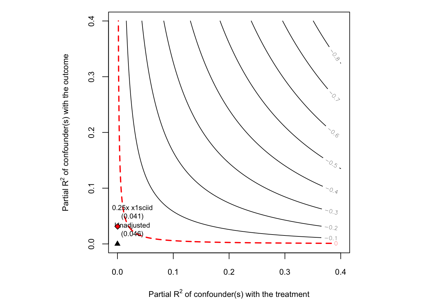
sen.m01 <-sensemakr(model = m01, treatment ="p2museumTreatment",benchmark_covariates ="x1sciid",kd =0.25:0.75, # strength of unobserved confounding with treatmentky =0.25:0.75, # strength of unobserve confounding with outcomeq =1, # threshold for nullifying the estimatealpha =0.05, # significance levelreduce =TRUE# test whether confounding could reduce effect )summary(sen.m01)
Sensitivity Analysis to Unobserved Confounding

Model Formula: x2sciid ~ x1sciid + p2museum + x1locale + x1control + x1region +
    a1mspdintrst + a1msmentor + x1race + x1sex + x1sesq5 + x1schoolbel +
    x1txmscr + x1sciint + x1stuedexpct + s1alg1m09 + s1sfall09 +
    p1campms + p1fixed + p1sciproj

Null hypothesis: q = 1 and reduce = TRUE
-- This means we are considering biases that reduce the absolute value of the current estimate.
-- The null hypothesis deemed problematic is H0:tau = 0

Unadjusted Estimates of 'p2museumTreatment':
  Coef. estimate: 0.0464
  Standard Error: 0.0227
  t-value (H0:tau = 0): 2.0456

Sensitivity Statistics:
  Partial R2 of treatment with outcome: 6e-04
  Robustness Value, q = 1: 0.0252
  Robustness Value, q = 1, alpha = 0.05: 0.0011

Verbal interpretation of sensitivity statistics:

-- Partial R2 of the treatment with the outcome: an extreme confounder (orthogonal to the covariates) that explains 100% of the residual variance of the outcome, would need to explain at least 0.06% of the residual variance of the treatment to fully account for the observed estimated effect.

-- Robustness Value, q = 1: unobserved confounders (orthogonal to the covariates) that explain more than 2.52% of the residual variance of both the treatment and the outcome are strong enough to bring the point estimate to 0 (a bias of 100% of the original estimate). Conversely, unobserved confounders that do not explain more than 2.52% of the residual variance of both the treatment and the outcome are not strong enough to bring the point estimate to 0.

-- Robustness Value, q = 1, alpha = 0.05: unobserved confounders (orthogonal to the covariates) that explain more than 0.11% of the residual variance of both the treatment and the outcome are strong enough to bring the estimate to a range where it is no longer 'statistically different' from 0 (a bias of 100% of the original estimate), at the significance level of alpha = 0.05. Conversely, unobserved confounders that do not explain more than 0.11% of the residual variance of both the treatment and the outcome are not strong enough to bring the estimate to a range where it is no longer 'statistically different' from 0, at the significance level of alpha = 0.05.

Bounds on omitted variable bias:

--The table below shows the maximum strength of unobserved confounders with association with the treatment and the outcome bounded by a multiple of the observed explanatory power of the chosen benchmark covariate(s).

   Bound Label R2dz.x R2yz.dx         Treatment Adjusted Estimate Adjusted Se
 0.25x x1sciid  3e-04  0.0314 p2museumTreatment             0.041      0.0223
 Adjusted T Adjusted Lower CI Adjusted Upper CI
     1.8378           -0.0027            0.0848
Code
plot(sen.m01 )
For non-weighted PS model + IPTW*sampl weight for outcome model
Code
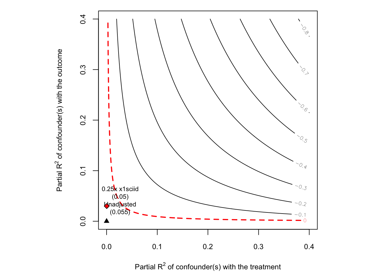
sen1 <-sensemakr(model = ate_dr_sciid, treatment ="p2museumTreatment",benchmark_covariates ="x1sciid",kd =0.25:0.75, # strength of unobserved confounding with treatmentky =0.25:0.75, # strength of unobserve confounding with outcomeq =1, # threshold for nullifying the estimatealpha =0.05, # significance levelreduce =TRUE# test whether confounding could reduce effect )summary(sen1)
Sensitivity Analysis to Unobserved Confounding

Model Formula: x2sciid ~ x1sciid + p2museum + x1locale + x1control + x1region +
    a1mspdintrst + a1msmentor + x1race + x1sex + x1sesq5 + x1schoolbel +
    x1txmscr + x1sciint + x1stuedexpct + s1alg1m09 + s1sfall09 +
    p1campms + p1fixed + p1sciproj

Null hypothesis: q = 1 and reduce = TRUE
-- This means we are considering biases that reduce the absolute value of the current estimate.
-- The null hypothesis deemed problematic is H0:tau = 0

Unadjusted Estimates of 'p2museumTreatment':
  Coef. estimate: 0.0555
  Standard Error: 0.0216
  t-value (H0:tau = 0): 2.5634

Sensitivity Statistics:
  Partial R2 of treatment with outcome: 0.001
  Robustness Value, q = 1: 0.0315
  Robustness Value, q = 1, alpha = 0.05: 0.0075

Verbal interpretation of sensitivity statistics:

-- Partial R2 of the treatment with the outcome: an extreme confounder (orthogonal to the covariates) that explains 100% of the residual variance of the outcome, would need to explain at least 0.1% of the residual variance of the treatment to fully account for the observed estimated effect.

-- Robustness Value, q = 1: unobserved confounders (orthogonal to the covariates) that explain more than 3.15% of the residual variance of both the treatment and the outcome are strong enough to bring the point estimate to 0 (a bias of 100% of the original estimate). Conversely, unobserved confounders that do not explain more than 3.15% of the residual variance of both the treatment and the outcome are not strong enough to bring the point estimate to 0.

-- Robustness Value, q = 1, alpha = 0.05: unobserved confounders (orthogonal to the covariates) that explain more than 0.75% of the residual variance of both the treatment and the outcome are strong enough to bring the estimate to a range where it is no longer 'statistically different' from 0 (a bias of 100% of the original estimate), at the significance level of alpha = 0.05. Conversely, unobserved confounders that do not explain more than 0.75% of the residual variance of both the treatment and the outcome are not strong enough to bring the estimate to a range where it is no longer 'statistically different' from 0, at the significance level of alpha = 0.05.

Bounds on omitted variable bias:

--The table below shows the maximum strength of unobserved confounders with association with the treatment and the outcome bounded by a multiple of the observed explanatory power of the chosen benchmark covariate(s).

   Bound Label R2dz.x R2yz.dx         Treatment Adjusted Estimate Adjusted Se
 0.25x x1sciid  3e-04    0.03 p2museumTreatment            0.0505      0.0213
 Adjusted T Adjusted Lower CI Adjusted Upper CI
     2.3677            0.0087            0.0923
Code
plot(sen1)
4. IPTW and Matching Comparsion
Matching vs Weighting
The Core Difference
Matching is like pruning a tree. You discard the observations that don’t have a “match” in the other group. You end up with a smaller, cleaner dataset where treated and control units look like twins.
Weighting is like sculpting clay. You keep everyone in the dataset, but you “stretch” (up-weight) or “squish” (down-weight) specific observations so that the total treated pile looks identical to the total control pile.
Feature
Matching
Weighting (IPTW)
Data Retention
Low. You often discard unmatched control units (and sometimes treated units), reducing sample size.
High. Uses the full sample (no data loss), which generally preserves statistical power.
Target Population
Changes. Usually estimates the ATT (effect on the treated) or a subset of it (the “matchable” treated).
Flexible. Can easily estimate ATE (whole population), ATT, or ATU depending on the formula used.
Extreme Values
Robust. Units with extreme propensity scores (no overlap) are simply dropped/ignored.
Sensitive. Units with extreme propensity scores get massive weights, causing unstable estimates and high variance.
Variance
Lower Variance (usually), but potentially higher bias if matches are poor.
Higher Variance, especially if weights are unstable (though “trimming” helps).
Interpretability
High. “We compared Student A to Student B who looked just like them.” Easy to explain to stakeholders.
Low. “We up-weighted Student A by 3.5x to represent a pseudo-population.” Harder to explain.
Balance Check
Must check balance after matching.
Must check balance after weighting.
References
Rosenbaum, P. R., & Rubin, D. B. (1983). The central role of the propensity score in observational studies for causal effects. Biometrika, 70(1), 41-55.
Stuart, E. A. (2010). Matching methods for causal inference: A review and a look forward. Statistical Science, 25(1), 1-21.
Guo, S., & Fraser, M. W. (2014). Propensity score analysis: Statistical methods and applications. Sage.
Austin, P. C. (2011). An introduction to propensity score methods for reducing the effects of confounding in observational studies. Multivariate Behavioral Research, 46(3), 399-424.
Imbens, G. W., & Wooldridge, J. M. (2009). Recent developments in the econometrics of program evaluation. Journal of Economic Literature, 47(1), 5-86.
Li, F., Morgan, K. L., & Zaslavsky, A. M. (2018). Balancing covariates via propensity score weighting. Journal of the American Statistical Association, 113(521), 390-400.
This tutorial is based on lecture materials from Stat 256: Causality (UCLA) and EDUC 255C: Introduction to Causal Inference in Education Research (UCLA), Spring 2025.
Source Code
---title: "Weighting Methods for Causal Inference"author: Shuhan (Alice) Aidate: "2025-05-10"categories: [R, Causal Inference]toc: truetoc-depth: 3toc-title: "Contents"code-fold: showcode-tools: trueimage: "f1.png"output: html_document: mathjax: default self_contained: true---In previous posts, we've explored the [Potential Outcomes framework](https://aliceaii.github.io/posts/ci_po/) and [matching methods](https://aliceaii.github.io/posts/ci_matching/) for causal inference. Today, we'll dive deeper into propensity score methods, which offer a powerful and flexible approach to addressing selection bias in observational studies.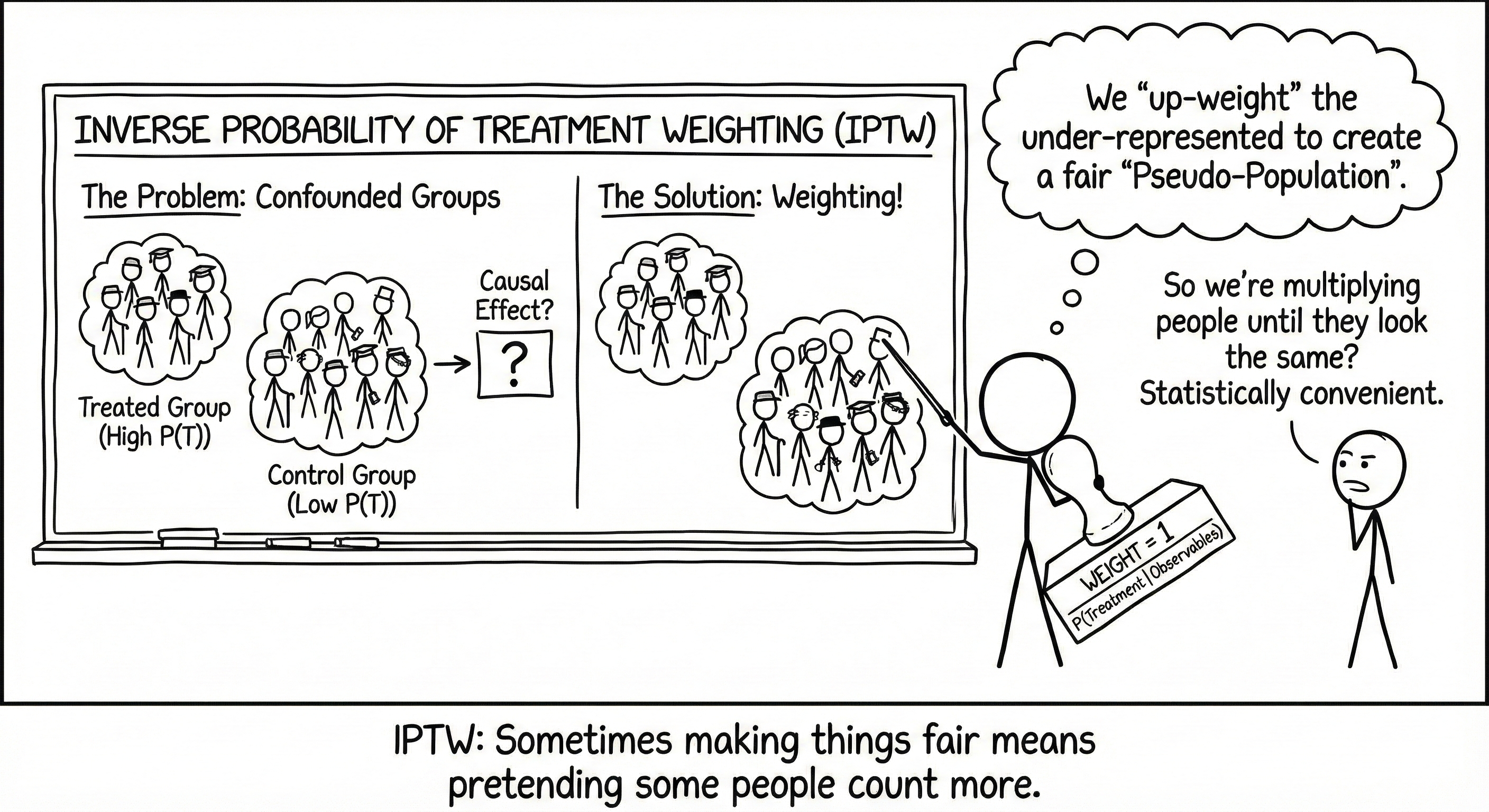## 1. IntroductionThe propensity score is defined as:$$p(X_i) = P(D_i = 1 | X_i)$$Where:- $D_i$ is the treatment indicator (1 if treated, 0 if control)- $X_i$ is a vector of observed covariates for unit $i$If we have two districts with the same propensity score, they have the same probability of receiving treatment based on their observed characteristics. This means that among districts with similar propensity scores, treatment assignment is assuming random - aiming to achieve a quasi-experimental design.A property of propensity scores is that if treatment assignment is strongly ignorable given $X$, then:$$Y_i(1), Y_i(0) \perp\!\!\!\perp D_i \mid \mathbf{X}_i$$This means that conditioning on the propensity score is sufficient to achieve independence between potential outcomes and treatment assignment. In other words, within strata of units with similar propensity scores, the distribution of covariates should be similar between treated and control groups.### 1.1 Propensity Score MethodsThere are three main ways to use propensity scores:1. **Matching**: Pair treated and control units with similar propensity scores2. **Inverse Probability of Treatment Weighting (IPTW)**: Weight observations by the inverse of their probability of receiving their observed treatment3. **Stratification**: Divide the sample into strata based on propensity score rangesIn this post, we'll focus on IPTW, with a practical example using educational data.## 2. Inverse Probability of Treatment Weighting (IPTW)### 2.1 Mathematical FoundationIPTW is based on creating a pseudo-population where treatment assignment is independent of confounders. The key insight is that by weighting each observation by the inverse of its probability of receiving the treatment it actually received, we can balance the covariate distributions between treatment groups.For the Average Treatment Effect (ATE), the weights are:$$w_i^{ATE} = \frac{D_i}{p(X_i)} + \frac{1-D_i}{1-p(X_i)}$$- For treated units ($D_i = 1$): $w_i = \frac{1}{p(X_i)}$- For control units ($D_i = 0$): $w_i = \frac{1}{1-p(X_i)}$For the Average Treatment Effect of Treated (ATT), the weights are:$$w_i^{ATT} = D_i + (1-D_i)\frac{p(X_i)}{1-p(X_i)}$$- For treated units ($D_i = 1$): $w_i = 1$- For control units ($D_i = 0$): $w_i = \frac{p(X_i)}{1-p(X_i)}$For the Average Treatment Effect of Untreated (ATU), the weights are:$$w_i^{ATU} = D_i\frac{1-p(X_i)}{p(X_i)} + (1-D_i)$$- For treated units ($D_i = 1$): $w_i = \frac{1-p(X_i)}{p(X_i)}$- For control units ($D_i = 0$): $w_i = 1$**Intuition Behind IPTW**The weights create a pseudo-population where:- Treated units who were unlikely to be treated (low $p(X_i)$) get high weights- Control units who were likely to be treated (high $p(X_i)$) get high weights- This "fills in" the missing counterfactuals by upweighting similar units from the opposite group## 3. HSLS:09 Science Museum Practical ExampleLeveraging the High School Longitudinal Study (HSLS:09), this example aims to answer the following questions:- **Treament:** What individual and contextual factors are associated with students’ likelihood of visiting science museums or planetariums during high school?- **Science Identity Formation:** Does participation in informal science learning experiences—such as visiting a science museum or planetarium between 9th and 11th grade—positively influence the development of a science identity?- **STEM Major Intentions:** Does exposure to science museums or planetariums during high school increase the likelihood of pursuing a STEM major in college?::: callout-noteThe analysis data file include 6,481 9th grade students with observed treatment group status and no-zero value of sample weight (W3W1W2STU).Missing rate range from 1% to 19%. Dealing with missing values using likewise deletion is problematic, given the sample size will be reduced considerably and will introduce bias unless the data is missing completely at random (Enders, 2010). In this study we impute single values using stochastic imputations and chained equations embedded in `mice` r package.The final analysis data file includes 8,106 college-bound students and the following variables:- `STU_ID` = unique HSLS student identifier (persistent 2009 – 2013)\- `SCH_ID` = unique HSLS school identifier (persistent 2009 – 2013)\- `W3W1W2STU` = W3 Student Longitudinal Analytic Weight BY-F1-U13\- `W1SCHOOL` = Baseline year school level Weight\**Treatment indicator:**\- `p2museum` = visited a science-related museum/planetarium between 9th and 11th grade (1 = Yes, 0 = No)\**Dependent variables (DVs):**\- `x2sciid` = 11th-grade science identity scale (standardized z-score)\- `collegeSTEMmajorasp` = binary indicator of whether the student aspired to or declared a STEM major while enrolled in college (1 = Yes, 0 = No)\**Pre-treatment covariates:**\- `x1sciid` = 9th-grade baseline science identity scale (standardized z-score)\- `stemoccasp9th` = binary indicator of whether the student aspired to a STEM occupation in 9th grade\**School-level covariates (baseline, 9th grade):**\- `x1locale` = school locale: City, Suburb, Town, Rural (ref)\- `x1control` = school control: Public, Catholic or other Private School (ref)\- `x1region` = U.S. census region of the school: Northeast (ref), Midwest, South, West\- `a1mspdintrst` = binary indicator for whether the school sponsored a math or science after-school program (Yes/No)\- `a1msmentor` = binary indicator for whether the school paired students with mentors in math or science (Yes/No)\**Student-level IVs: background characteristics:**\- `x1race` = White (ref), Asian, Black, Latino, Multiracial, Native American, Other\- `x1sex` = binary sex indicator (0 = Male, 1 = Female)\- `x1sesq5` = socioeconomic status quintile, First quintile (ref, lowest), Second, Third, Fourth, and Fifth quintile (highest)\- `x1txmscr` = 9th-grade math achievement score (IRT-scaled)\- `x1sciint` = science course interest scale (standardized z-score)\- `x1stuedexpct` = student's highest educational expectation, categorized as Uncertain (ref), High School, Bachelor’s, Master’s, or PhD\- `x1schoolbel` = 9th-grade student-perceived school belonging scale (standardized z-score)\**Student-leve IVs: formal and informal STEM experiences (9th grade):**\- `s1alg1m09` = binary indicator of whether the student took Algebra I in 9th grade (Yes/No)\- `s1sfall09` = binary indicator of whether the student took a science course in fall 2009 (Yes/No)\- `p1campms` = binary indicator of whether the student participated in math or science camp outside of school in last year (Yes/No)\- `p1fixed` = binary indicator of whether parents built or fixed something with 9th grader in last year (Yes/No)\- `p1sciproj` = binary indicator of whether the helped 9th grader with a school science fair project in last year with 9th grader in last year (Yes/No)\Analysis the outcome, ATE, ATT, ATU:- Used doubly robust approach- Consider using MLM random slop (two levels: student level and school level)- Then conduct robustness check, use sensemakr to run the sensitivity analysis- Use student’s 9th grade science identity as benchmark covariates:::```{r, warning=FALSE, message=FALSE}rm(list =ls())library(tidyverse)library(skimr)library(flextable)library(table1)library(tableone)library(knitr)library(MatchIt)library(WeightIt)library(cobalt) #for love plots library(marginaleffects)library(sensemakr) #sensitivity analysislibrary(patchwork)library(car)library(naniar)library(mice)library(haven)library(lm.beta) #standardized beta coef (for comparing effect sizes)library(lme4) #for fixed modelslibrary(survey) #for weights and robust SEslibrary(broom) #convert model into tidy data frameslibrary(lme4)library(merTools)library(lmerTest)library(WeMix) data <-readRDS("hslspsm_imputed.rds")```### 3.1 Descriptive Analysis```{r, warning=FALSE, message=FALSE}length(unique(data$STU_ID))length(unique(data$SCH_ID))autofit(as_flextable(table(data$p2museum)))#combine Native American and Other other all into others categories due to small subpopulationdata <- data %>%mutate(x1race =fct_collapse(x1race,Other =c("Native American", "Other") # <- names to merge ))#Descriptive Analysisdescr1 <-table1(~ x1sciid + stemoccasp9th +#pre-IVs x1locale + x1control + x1region + a1mspdintrst + a1msmentor +#school-level IV x1race + x1sex + x1sesq5 + x1schoolbel + x1txmscr + x1sciint + x1stuedexpct +#student-level IV background s1alg1m09 + s1sfall09 + p1campms + p1fixed + p1sciproj + x2sciid + collegeSTEMmajorasp |as.factor(p2museum), data = data)descr1```#### Compute the navie effect without adding PS and Weighting##### Unconditional Navie Estimate (No PS, no sample weight, single level without covaraite adjustment)```{r, warning=FALSE, message=FALSE}m00 <-lm(x2sciid ~ p2museum, data = data)summary(m00)sqrt(hccm(m00)[2,2])m000 <-glm(collegeSTEMmajorasp ~ p2museum, data = data, family ="binomial" )summary(m000)``````{r, include=FALSE, warning=FALSE, message=FALSE}#write function to create coefficient table - lineartidy.coeftable <-function(model, digits =3) {# Model summary model_summary <-summary(model)# Extract coefficients, SEs, p-values b <- model_summary$coefficients[, "Estimate"] se <- model_summary$coefficients[, "Std. Error"] pval <- model_summary$coefficients[, "Pr(>|t|)"]# Get standardized betas beta <-lm.beta(model)$standardized.coefficients# Significance stars get_stars <-function(p) {if (is.na(p)) return("")elseif (p <0.001) return("***")elseif (p <0.01) return("**")elseif (p <0.05) return("*")elseif (p <0.1) return(".")elsereturn("") } stars <-sapply(pval, get_stars)# Combine everything into a data frame coef_table <-data.frame(Variable =names(b),Coefficient =round(b, digits),SE =round(se, digits),Beta =round(beta, digits),p_value =round(pval, digits),Sig = stars,row.names =NULL )return(coef_table)}#write function to create coefficient table - logistictidy.logit.table <-function(model, digits =3) {# Get model summary model_summary <-summary(model)# Extract unstandardized log-odds coefficients b <- model_summary$coefficients[, "Estimate"] se <- model_summary$coefficients[, "Std. Error"] pval <- model_summary$coefficients[, "Pr(>|z|)"]# Compute odds ratios and CI OR <-exp(b)# Significance stars get_stars <-function(p) {if (is.na(p)) return("")elseif (p <0.001) return("***")elseif (p <0.01) return("**")elseif (p <0.05) return("*")elseif (p <0.1) return(".")elsereturn("") } stars <-sapply(pval, get_stars)# Combine results coef_table <-data.frame(Variable =names(b),Coefficient =round(b, digits),SE =round(se, digits),OR =round(OR, digits),p_value =round(pval, digits),Sig = stars )return(coef_table)}```##### Navie Estimate (No PS, no sample weight, single level with covaraite adjustment)```{r, warning=FALSE, message=FALSE}m01 <-lm(x2sciid ~ x1sciid +#pre-IVs p2museum + x1locale + x1control + x1region + a1mspdintrst + a1msmentor +#school-level IV x1race + x1sex + x1sesq5 + x1schoolbel + x1txmscr + x1sciint + x1stuedexpct +#student-level IV background s1alg1m09 + s1sfall09 + p1campms + p1fixed + p1sciproj, data = data)sqrt(hccm(m01)[3,3]) #HC2 robust sd for treatmenttable.m01<-tidy.coeftable(m01)knitr::kable(table.m01, digits =3, caption ="Unweighted multiple linear regression results predicting 11th science identity")m001 <-glm(collegeSTEMmajorasp ~ stemoccasp9th +#pre-IVs p2museum +#treatment x1locale + x1control + x1region + a1mspdintrst + a1msmentor +#school-level IV x1race + x1sex + x1sesq5 + x1schoolbel + x1txmscr + x1sciint + x1stuedexpct +#student-level IV background s1alg1m09 + s1sfall09 + p1campms + p1fixed + p1sciproj, data = data, family ="binomial" )table.m001 <-tidy.logit.table(m001)knitr::kable(table.m001, digits =3, caption ="Unweighted multiple logistic regression results predicting STEM major aspiration")```### 3.2 Define Distance Measure - Propensity score - glm#### Proposentity score without sample weight```{r, warning=FALSE, message=FALSE}#estimate logistic modelpscore.m <-glm(p2museum ~ x1sciid + stemoccasp9th +#pre-IVs x1locale + x1control + x1region + a1mspdintrst + a1msmentor +#school-level IV x1race + x1sex + x1sesq5 + x1schoolbel + x1txmscr + x1sciint + x1stuedexpct +#student-level IV background s1alg1m09 + s1sfall09 + p1campms + p1fixed + p1sciproj, data = data, family ="binomial")table.pscore.m <-tidy.logit.table(pscore.m)knitr::kable(table.pscore.m, digits =3, caption ="Multiple logistic regression results predicting science museum or or planetariums visit")#get predicted probabilities/and probabilies on log-odds scaledata <- data %>%mutate(pscore =predict(pscore.m, type ="response"),pscorelogodd =predict(pscore.m))#summary(data$pscorelogodd[data$p2museum == "Treatment"])#summary(data$pscorelogodd[data$p2museum == "Control"])#summary(data$pscore[data$p2museum == "Treatment"])#summary(data$pscore[data$p2museum == "Control"])```##### Examine Common Support (overlap) without weight```{r, warning=FALSE, message=FALSE}#examine common support(overlap)#create plotsp1 <-ggplot(data, aes(x = pscore, fill = p2museum)) +geom_histogram(binwidth =0.01, position ="identity", alpha =0.6, color ="black") +scale_fill_manual(values =c("#ee84a8", "#71bced"), labels =c("Control", "Treatment")) +labs(title ="Propensity Score (Linear Scale)", x ="Propensity Score", y ="Frequency", fill ="Science Museum") +theme_minimal() +theme(plot.title =element_text(size =12))p2 <-ggplot(data, aes(x = pscore, y = p2museum, color = p2museum)) +geom_jitter(height =0.2, alpha =0.4, size =1) +scale_color_manual(values =c("#ee84a8", "#71bced"), labels =c("Control", "Treatment")) +labs(title ="Common Support by Group", x ="Propensity Score", y =NULL, color ="Science Museum") +theme_minimal() +theme(plot.title =element_text(size =12))p3 <-ggplot(data, aes(x = pscorelogodd, y = p2museum, color = p2museum)) +geom_jitter(height =0.2, alpha =0.4, size =1) +scale_color_manual(values =c("#ee84a8", "#71bced"), labels =c("Control", "Treatment")) +scale_x_continuous(breaks =seq(floor(min(data$pscorelogodd, na.rm =TRUE)),ceiling(max(data$pscorelogodd, na.rm =TRUE)), by =0.2)) +labs(title ="Common Support by Group", x ="Logit Score", y =NULL, color ="Science Museum") +theme_minimal() +theme(plot.title =element_text(size =12))#combine allcombined_plot <- p1 / p2 / p3 +plot_layout(ncol =1, heights =c(4, 3, 3))combined_plot```##### Trim the data PS without weight```{r, warning=FALSE, message=FALSE}table(data$STU_ID[data$pscorelogodd <-1.6])table(data$STU_ID[data$pscorelogodd >1.0])data_trimmed <- data %>%filter(pscorelogodd >=-1.6& pscorelogodd <=1.0)table(data_trimmed$p2museum)#total loss 41 cases```### 3.3 IPTW, balance with IPTW\*W3W1W2STUCompare two weight methods:- First, use non-weighted PSM, them multiply by the ate/att/atc, we get: w.ate_W3W1W2STU; w.att_W3W1W2STU; w.atc_W3W1W2STU- Second, use sample weight in the propensity score stage, then compute final weights as the product of the sampling weight and the propensity score weight: w.ate.w_W3W1W2STU; w.att.w_W3W1W2STU; w.atc.w_W3W1W2STU.#### Combined weight with non-weighted PSM```{r, warning=FALSE, message=FALSE}#normalize the panel weightdata_trimmed <- data_trimmed %>%mutate(W3W1W2STU_norm = W3W1W2STU /mean(W3W1W2STU, na.rm =TRUE))#calculate IPTW (ATE, ATT, ATU)data_trimmed <- data_trimmed %>%#weight based on the treatmentmutate(D =ifelse(p2museum =="Treatment", 1, 0),w.ate = (D * (1/pscore)) + ((1- D) * (1/(1- pscore))),w.att = (D) + ((1- D) * (pscore/(1- pscore))),w.atc = (D * ((1- pscore)/pscore)) + (1- D),#balance the weight based on the control levelw.ate_W3W1W2STU = w.ate*W3W1W2STU_norm,w.att_W3W1W2STU = w.att*W3W1W2STU_norm,w.atc_W3W1W2STU = w.atc*W3W1W2STU_norm )table(data_trimmed$D)table(data_trimmed$p2museum)```##### Check the data balanceSMD is \<0.10 for all covariates```{r, warning=FALSE, message=FALSE}#question? check the balance only for w.ate or for w.ate_W3W1W2STUcovars <-c("x1sciid", "x1locale", "x1control", "x1region", "a1mspdintrst", "a1msmentor","x1race", "x1sex", "x1sesq5", "x1schoolbel", "x1txmscr", "x1sciint", "x1stuedexpct", "s1alg1m09", "s1sfall09","p1campms", "p1fixed", "p1sciproj") bal_ate <-bal.tab(x = data_trimmed[, covars],treat = data_trimmed$D,weights = data_trimmed$w.ate_W3W1W2STU,estimand ="ATE",s.d.denom ="pooled", # std-diff denominatorm.threshold = .1, # ±0.10 rule of thumbun =TRUE)bal_ate#questions? what's the Effective sample sizes mean here?#The effective numbers after applying the IPTW*W3W1W2STU weights had a sample of about 1,574 controls and 959 treated cases.love.plot(bal_ate,stats ="mean.diffs",abs =FALSE, binary ="std", thresholds =c(m = .10),colors =c("#ee84a8", "#71bced"),title ="Covariate Balance after IPTW (ATE)") +theme_bw()```##### Get the descriptive stats after weighting (ATE)```{r, warning=FALSE, message=FALSE}#create survey design object using IPTW weightsdesign <-svydesign(ids =~1, weights =~w.ate_W3W1W2STU, data = data_trimmed)#create post-weighting descriptive table by treatment grouptable_weighted <-svyCreateTableOne(vars = covars, strata ="p2museum", data = design)print(table_weighted)```### 3.4 ATE, ATT, ATC#### Nested Result with IPW science identity```{r, warning=FALSE, message=FALSE}#estimate navie ATE of museum on sciidate_sciid <-lm(x2sciid ~ x1sciid +#pre-IVs p2museum, data = data_trimmed, weights = w.ate_W3W1W2STU)sqrt(hccm(ate_sciid)[3,3])table.ate_sciid <-tidy.coeftable(ate_sciid) knitr::kable(table.ate_sciid, digits =3, caption ="nested1 ATE weighted results of linear regression on science identity")ate_sciid2 <-lm(x2sciid ~ x1sciid +#pre-IVs p2museum + x1locale + x1control + x1region + a1mspdintrst + a1msmentor + x1race + x1sex + x1sesq5 + x1schoolbel + x1txmscr + x1sciint + x1stuedexpct, data = data_trimmed, weights = w.ate_W3W1W2STU)sqrt(hccm(ate_sciid2)[3,3])table.ate_sciid2 <-tidy.coeftable(ate_sciid2)knitr::kable(table.ate_sciid2, digits =3, caption ="nested 2 ATE weighted results of linear regression on science identity")```#### Result with IPW science identity```{r, warning=FALSE, message=FALSE}#estimate ATE of museum on sciidate_dr_sciid <-lm(x2sciid ~ x1sciid +#pre-IVs p2museum + x1locale + x1control + x1region + a1mspdintrst + a1msmentor +#school-level IV x1race + x1sex + x1sesq5 + x1schoolbel + x1txmscr + x1sciint + x1stuedexpct +#student-level IV background s1alg1m09 + s1sfall09 + p1campms + p1fixed + p1sciproj, data = data_trimmed, weights = w.ate_W3W1W2STU)sqrt(hccm(ate_dr_sciid)[3,3])table.ate_dr_sciid <-tidy.coeftable(ate_dr_sciid)knitr::kable(table.ate_dr_sciid, digits =3, caption ="ATE weighted results of linear regression on science identity")#estimate ATT of museum on sciidatt_dr_sciid <-lm(x2sciid ~ x1sciid +#pre-IVs p2museum + x1locale + x1control + x1region + a1mspdintrst + a1msmentor +#school-level IV x1race + x1sex + x1sesq5 + x1schoolbel + x1txmscr + x1sciint + x1stuedexpct +#student-level IV background s1alg1m09 + s1sfall09 + p1campms + p1fixed + p1sciproj, data = data_trimmed, weights = w.att_W3W1W2STU)sqrt(hccm(att_dr_sciid)[3,3])table.att_dr_sciid <-tidy.coeftable(att_dr_sciid)knitr::kable(table.att_dr_sciid, digits =3, caption ="ATT weighted results of linear regression on science identity")#estimate ATC of museum on sciidatc_dr_sciid <-lm(x2sciid ~ x1sciid +#pre-IVs p2museum + x1locale + x1control + x1region + a1mspdintrst + a1msmentor +#school-level IV x1race + x1sex + x1sesq5 + x1schoolbel + x1txmscr + x1sciint + x1stuedexpct +#student-level IV background s1alg1m09 + s1sfall09 + p1campms + p1fixed + p1sciproj, data = data_trimmed, weights = w.atc_W3W1W2STU)sqrt(hccm(atc_dr_sciid)[3,3])table.atc_dr_sciid <-tidy.coeftable(atc_dr_sciid)knitr::kable(table.atc_dr_sciid, digits =3, caption ="ATC weighted results of linear regression on science identity")```#### Nested Result with IPW STEM Major Asp```{r, warning=FALSE, message=FALSE}ate_stemma <-glm(collegeSTEMmajorasp ~ stemoccasp9th + p2museum,data = data_trimmed, family =binomial(), weights = w.ate_W3W1W2STU)table.ate_stemma <-tidy.logit.table(ate_stemma)knitr::kable(table.ate_stemma, digits =3, caption ="nested1 ATE weighted multiple logistic regression results of STEM major aspiration")ate_stemma2 <-glm(collegeSTEMmajorasp ~ stemoccasp9th +#pre-IVs p2museum + x1locale + x1control + x1region + a1mspdintrst + a1msmentor + x1race + x1sex + x1sesq5 + x1schoolbel + x1txmscr + x1sciint + x1stuedexpct,data = data_trimmed, family =binomial(), weights = w.ate_W3W1W2STU)table.ate_stemma2 <-tidy.logit.table(ate_stemma2)knitr::kable(table.ate_stemma2, digits =3, caption ="nested2 ATE weighted multiple logistic regression results of STEM major aspiration")```#### Result with IPW STEM Major Asp```{r, warning=FALSE, message=FALSE}#estimate ATE of museum on STEM major# Outcome model with doubly robust estimator using ATE weightsate_dr_stemma <-glm(collegeSTEMmajorasp ~ stemoccasp9th +#pre-IVs p2museum + x1locale + x1control + x1region + a1mspdintrst + a1msmentor +#school-level IV x1race + x1sex + x1sesq5 + x1schoolbel + x1txmscr + x1sciint + x1stuedexpct +#student-level IV background s1alg1m09 + s1sfall09 + p1campms + p1fixed + p1sciproj,data = data_trimmed, family =binomial(), weights = w.ate_W3W1W2STU)table.ate_dr_stemma <-tidy.logit.table(ate_dr_stemma)knitr::kable(table.ate_dr_stemma, digits =3, caption ="ATE weighted multiple logistic regression results of STEM major aspiration")# Outcome model with doubly robust estimator using ATT weightsatt_dr_stemma <-glm(collegeSTEMmajorasp ~ stemoccasp9th +#pre-IVs p2museum + x1locale + x1control + x1region + a1mspdintrst + a1msmentor +#school-level IV x1race + x1sex + x1sesq5 + x1schoolbel + x1txmscr + x1sciint + x1stuedexpct +#student-level IV background s1alg1m09 + s1sfall09 + p1campms + p1fixed + p1sciproj,data = data_trimmed, family =binomial(), weights = w.att_W3W1W2STU)table.att_dr_stemma <-tidy.logit.table(att_dr_stemma)knitr::kable(table.ate_dr_stemma, digits =3, caption ="ATT weighted multiple logistic regression results of STEM major aspiration")# Outcome model with doubly robust estimator using ATU weightsatc_dr_stemma <-glm(collegeSTEMmajorasp ~ stemoccasp9th +#pre-IVs p2museum + x1locale + x1control + x1region + a1mspdintrst + a1msmentor +#school-level IV x1race + x1sex + x1sesq5 + x1schoolbel + x1txmscr + x1sciint + x1stuedexpct +#student-level IV background s1alg1m09 + s1sfall09 + p1campms + p1fixed + p1sciproj,data = data_trimmed, family =binomial(), weights = w.atc_W3W1W2STU)table.atc_dr_stemma <-tidy.logit.table(atc_dr_stemma)knitr::kable(table.atc_dr_stemma, digits =3, caption ="ATC weighted multiple logistic regression results of STEM major aspiration")```### 3.5 ATE in MLM#### For unweighted PSICC for the end of 11th sciid is 5%.```{r, warning=FALSE, message=FALSE}#convert the SCH_ID into a fdata_trimmed$SCH_ID <-as.factor(data_trimmed$SCH_ID)#run the unconditional model m0_mlm <-lmer(x2sciid ~1+ (1| SCH_ID), data = data_trimmed, weights = w.ate_W3W1W2STU)summary(m0_mlm)#icc for sciid is 5%icc0 <-0.09/ (0.09+1.73)icc0```### 3.6 Heterogenity, Moderation Effect by Race and Gender##### Applied for unweighted PS model + (IPW\*sample weight) for single level outcome model```{r, warning=FALSE, message=FALSE}#estimate ATE Heterogenity on Race and Gender of museum on sciidate_dr_sciid_hete <-lm(x2sciid ~ x1sciid +#pre-IVs p2museum + x1locale + x1control + x1region + a1mspdintrst + a1msmentor +#school-level IV x1race + x1sex + x1sesq5 + x1schoolbel + x1txmscr + x1sciint + x1stuedexpct +#student-level IV background s1alg1m09 + s1sfall09 + p1campms + p1fixed + p1sciproj + p2museum:x1race + p2museum:x1sex, data = data_trimmed, weights = w.ate_W3W1W2STU)table.ate_dr_sciid_hete <-tidy.coeftable(ate_dr_sciid_hete)knitr::kable(table.ate_dr_sciid_hete, digits =3, caption ="Racial and gender variation in science club effects on science identity")```### 3.7 Sensitivity Analysis#### For Navie Estimate (No PS, no sample weight, single level with covaraite adjustment)```{r, warning=FALSE, message=FALSE}sen.m01 <-sensemakr(model = m01, treatment ="p2museumTreatment",benchmark_covariates ="x1sciid",kd =0.25:0.75, # strength of unobserved confounding with treatmentky =0.25:0.75, # strength of unobserve confounding with outcomeq =1, # threshold for nullifying the estimatealpha =0.05, # significance levelreduce =TRUE# test whether confounding could reduce effect )summary(sen.m01)plot(sen.m01 )```#### For non-weighted PS model + IPTW\*sampl weight for outcome model```{r, warning=FALSE, message=FALSE}sen1 <-sensemakr(model = ate_dr_sciid, treatment ="p2museumTreatment",benchmark_covariates ="x1sciid",kd =0.25:0.75, # strength of unobserved confounding with treatmentky =0.25:0.75, # strength of unobserve confounding with outcomeq =1, # threshold for nullifying the estimatealpha =0.05, # significance levelreduce =TRUE# test whether confounding could reduce effect )summary(sen1)plot(sen1)```## 4. IPTW and Matching Comparsion**Matching vs Weighting**The Core Difference- **Matching** is like **pruning a tree**. You discard the observations that don't have a "match" in the other group. You end up with a smaller, cleaner dataset where treated and control units look like twins.- **Weighting** is like **sculpting clay**. You keep everyone in the dataset, but you "stretch" (up-weight) or "squish" (down-weight) specific observations so that the total treated pile looks identical to the total control pile.| Feature | Matching | Weighting (IPTW) || :---| :---| :---|| **Data Retention** | **Low.** You often discard unmatched control units (and sometimes treated units), reducing sample size. | **High.** Uses the full sample (no data loss), which generally preserves statistical power. || **Target Population** | **Changes.** Usually estimates the ATT (effect on the treated) or a subset of it (the "matchable" treated). | **Flexible.** Can easily estimate ATE (whole population), ATT, or ATU depending on the formula used. || **Extreme Values** | **Robust.** Units with extreme propensity scores (no overlap) are simply dropped/ignored. | **Sensitive.** Units with extreme propensity scores get massive weights, causing unstable estimates and high variance. || **Variance** | **Lower Variance** (usually), but potentially higher bias if matches are poor. | **Higher Variance**, especially if weights are unstable (though "trimming" helps). || **Interpretability** | **High.** "We compared Student A to Student B who looked just like them." Easy to explain to stakeholders. | **Low.** "We up-weighted Student A by 3.5x to represent a pseudo-population." Harder to explain. || **Balance Check** | Must check balance *after* matching. | Must check balance *after* weighting. |## References- Rosenbaum, P. R., & Rubin, D. B. (1983). The central role of the propensity score in observational studies for causal effects. *Biometrika*, 70(1), 41-55.- Stuart, E. A. (2010). Matching methods for causal inference: A review and a look forward. *Statistical Science*, 25(1), 1-21.- Guo, S., & Fraser, M. W. (2014). *Propensity score analysis: Statistical methods and applications*. Sage.- Austin, P. C. (2011). An introduction to propensity score methods for reducing the effects of confounding in observational studies. *Multivariate Behavioral Research*, 46(3), 399-424.- Imbens, G. W., & Wooldridge, J. M. (2009). Recent developments in the econometrics of program evaluation. *Journal of Economic Literature*, 47(1), 5-86.- Li, F., Morgan, K. L., & Zaslavsky, A. M. (2018). Balancing covariates via propensity score weighting. *Journal of the American Statistical Association*, 113(521), 390-400.---*This tutorial is based on lecture materials from Stat 256: Causality (UCLA) and EDUC 255C: Introduction to Causal Inference in Education Research (UCLA), Spring 2025.*