Predicting STEM Undergraduates’ Intentions to Pursue Scientific Research Careers

This document presents the results and R analyses for the STATS 202A final project

0. Introduction

• limit the sample to STEM bachelor degree recipient
• missing values rate, mice
• outliers

Also prepare the variables lists here…

• SCICAREER (outcome): Will you puruse a science-related research career? 5-point(1=Definitely no; 2=Probably no; 3=Uncertain; 4=Probably yes; 5=Definitely yes);binary (1 = Yes, 0 = otherwise)

• Science identity (continous): A measure describing the extent to which students conceive of themselves as scientists.

• Science self-efficacy (continuous): Measure of students’ confidence in their ability to conduct scientific research.

• Academic self-concept (continous): A measure of students’ beliefs about their abilities and confidence in academic environments.

• Habits of minds (continous): A measure of the behaviors and traits associated with academic success. These behaviors are seen as the foundation for lifelong learning.

• MAJORGPA: 1=D; 2=C; 3=C+; 4=B-; 5=B; 6=B+; 7=A-; 8=A or A+

• GOAL19: Goal: Making a theoretical contribution to science (1=Not Important; 2=Somewhat Important; 3=Very Important; 4=Essential)

• GOAL11: Goal: Helping others who are in difficulty

• GOAL04: Goal: Becoming an authority in my field

• RESEARCH: How many months since entering college (including summer) did you work on a professor’s research project? (1=0 months; 2=1-3 months; 3=4-6 months; 4=7-12 months; 5=13-24 months; 6=25+ months)

• HPW17: Hours per Week: Studying/homework. During the past year, how much time did you spend during a typical week: (1=None; 2=Less than 1 hour; 3=1-2; 4=3-5; 5=6-10; 6=11-15; 7=16-20; 8=Over 20)

• HPW29: Hours per Week: Studying with other students

• HPW28: Hours per Week: Socializing with friends in person

• HPW09: Hours per Week: Using social media

• HPW04: Hours per Week: Participating in student clubs/groups

• HPW24: Hours per Week: Watching TV/online video content (e.g., Amazon, Hulu, Netflix, YouTube)

• HPW06: Hours per Week: Exercising/sports

• HPW27: Hours per Week: Working (for pay) on campus

• HPW02:Hours per Week: Career planning (job searches, networking, etc.)

Methods

• descriptive analysis, cross-tabulations, raw data (with jitter) overlaid with Box

• Linear regression, model diagnosis

• Univariate Kernel Density Estimation

• Kernel Regression Estimation

• Prediction Model

load the data

rm(list = ls())
library(tidyverse)
library(dplyr)
library(skimr)
library(haven)
library(table1)
library(mice)
library(ggplot2)
library(patchwork)  
library(scales) 
library(lattice)
library(gridExtra)

data <- read_sav("/Users/aishuhan/Desktop/CCW and Undergraduate WOC STEM Career/CSS2019.SAV")
dim(data)

[1] 11776   677

dt <- data %>%
  select(MAJOR1, STUID, SCICAREER, 
         SCIENCE_SELF_EFFICACY, SCIENCE_IDENTITY, ACADEMIC_SELFCONCEPT, HABITS_OF_MIND,
         MAJORGPA, GOAL19, GOAL11, GOAL04, RESEARCH,
         HPW17, HPW29, HPW28, HPW09, HPW04, HPW24, HPW06, HPW27, HPW02)

head(dt)

# A tibble: 6 × 21
  MAJOR1                  STUID SCICAREER SCIENCE_SELF_EFFICACY SCIENCE_IDENTITY
  <dbl+lbl>               <chr> <dbl+lbl>                 <dbl>            <dbl>
1   1 [Art, fine and app… 9892… 3 [Uncer…                  65.0             48.6
2 114 [Biochemistry/Biop… 9892… 3 [Uncer…                  46.8             55.2
3   3 [English (language… 9892… 1 [Defin…                  39.7             33.4
4   4 [History]           9891… 1 [Defin…                  42.8             43.6
5   7 [Music]             9892… 2 [Proba…                  48.6             43.3
6  11 [Other Arts and Hu… 9892… 4 [Proba…                  51.2             52.5
# ℹ 16 more variables: ACADEMIC_SELFCONCEPT <dbl>, HABITS_OF_MIND <dbl>,
#   MAJORGPA <dbl+lbl>, GOAL19 <dbl+lbl>, GOAL11 <dbl+lbl>, GOAL04 <dbl+lbl>,
#   RESEARCH <dbl+lbl>, HPW17 <dbl+lbl>, HPW29 <dbl+lbl>, HPW28 <dbl+lbl>,
#   HPW09 <dbl+lbl>, HPW04 <dbl+lbl>, HPW24 <dbl+lbl>, HPW06 <dbl+lbl>,
#   HPW27 <dbl+lbl>, HPW02 <dbl+lbl>

#str(dt)

dt <- dt %>%
  mutate(
    major = case_when(
      MAJOR1 %in% c(112, 113, 114, 115, 116, 117, 118, 119, 120, 121, 122, 123) ~ 1,  # Bio & Life Sci
      MAJOR1 %in% c(663, 664, 665) ~ 2,                                               # Math & CS
      MAJOR1 %in% c(442, 443, 444, 445, 446, 447, 448, 449, 450, 451, 452, 453, 454) ~ 3,  # Engineering
      MAJOR1 %in% c(766, 767, 768, 769, 770, 771, 772) ~ 4,                          # Physical Sci
      MAJOR1 %in% c(555, 556, 557, 558, 559, 560, 561, 562) ~ 5,                    # Health Professions
      !is.na(MAJOR1) ~ 0,  # Non-STEM: any valid MAJOR1 value not in the above categories
      TRUE ~ NA_real_
    ),
    major = factor(major,
                        levels = c(0, 1, 2, 3, 4, 5), 
                        labels = c("non-STEM",
                                   "Health Professions",
                                   "Biological & Life Sciences",
                                   "Math & Computer Science",
                                   "Engineering",
                                   "Physical Science")))
dim(dt)    

[1] 11776    22

check missingness and outliers

The missing rate is less than 1.6%, the Little’s MCAR test is non significant, suggesting the missingness appears random and not systematically related to observed values. So I used the likewise deletion here.

For the outcome variables, since it’s a continues variables, I standardized them removed those cases have |z|>3.0. Removed 22 outliers.

For those ordinal variables using 3/4/5 points Likert responses, so I don’t remove or Winsorize anything.

#filter students who have non-missing outcome variable
dt <- dt %>% filter(!is.na(MAJOR1), !is.na(SCICAREER))

dt %>% summarise(across(everything(), ~ mean(is.na(.)))) 

# A tibble: 1 × 22
  MAJOR1 STUID SCICAREER SCIENCE_SELF_EFFICACY SCIENCE_IDENTITY
   <dbl> <dbl>     <dbl>                 <dbl>            <dbl>
1      0     0         0                0.0190           0.0163
# ℹ 17 more variables: ACADEMIC_SELFCONCEPT <dbl>, HABITS_OF_MIND <dbl>,
#   MAJORGPA <dbl>, GOAL19 <dbl>, GOAL11 <dbl>, GOAL04 <dbl>, RESEARCH <dbl>,
#   HPW17 <dbl>, HPW29 <dbl>, HPW28 <dbl>, HPW09 <dbl>, HPW04 <dbl>,
#   HPW24 <dbl>, HPW06 <dbl>, HPW27 <dbl>, HPW02 <dbl>, major <dbl>

#run Little's MCAR test
library(MissMech)
dt.c <- dt[, -c(1, 2, 3,22)]
#TestMCARNormality(dt.c)

#check outliers, remove cases with z-scores beyond ±3
dt <- dt %>% 
  mutate(SCIENCE_SELF_EFFICACY_z = scale(SCIENCE_SELF_EFFICACY)[,1],
         SCIENCE_IDENTITY_z = scale(SCIENCE_IDENTITY)[,1],
         ACADEMIC_SELFCONCEPT_z = scale(ACADEMIC_SELFCONCEPT)[,1],
         HABITS_OF_MIND_z = scale(HABITS_OF_MIND)[,1])

#listwise deletion and filter the sample to only include STEM students
dt <- dt %>% 
  drop_na() %>%
  filter(major != "non-STEM") %>%
  filter(abs(SCIENCE_SELF_EFFICACY_z) <= 3.0 &
         abs(SCIENCE_IDENTITY_z) <= 3.0 &
         abs(ACADEMIC_SELFCONCEPT_z) <= 3.0 &
         abs(HABITS_OF_MIND_z) <= 3.0)
#write.csv(dt, "dt_cleaned.csv", row.names = FALSE)

1. Descriptive & Linear

sample

#skim(dt)
table1(~ factor(SCICAREER) + factor(major) + SCIENCE_SELF_EFFICACY + SCIENCE_IDENTITY + 
         ACADEMIC_SELFCONCEPT +  HABITS_OF_MIND +
         MAJORGPA + GOAL19 + GOAL11 + GOAL04 + RESEARCH +
         HPW17 + HPW29 + HPW28 + HPW09 + HPW04 + HPW24 + HPW06 + HPW27 + HPW02, data = dt)

box-plot

Box plot of science-related research aspirations/science self-efficacay/GOAL19/RESEARCH by major.

major_colors <- c("Health Professions" = "#B7B7EB","Biological & Life Sciences" = "#56B4E9",
       "Math & Computer Science" = "#009E73","Engineering" = "#F0E442", "Physical Science" = "#F09BA0")

p0 <- ggplot(dt, aes(x = major, y = as.numeric(SCICAREER), fill = major)) +
  geom_jitter(width = 0.2, alpha = 0.3, size = 1, color = "gray45", shape = 16) +
  geom_boxplot(alpha = 0.6, outlier.shape = NA, width = 0.6) +
  scale_fill_manual(values = major_colors) +
  scale_y_continuous(breaks = 1:5, 
       labels = c("Definitely no", "Probably no", "Uncertain", "Probably yes", "Definitely yes")) +
  labs(title = "Scientific Research Careers Aspirations by Major", y = NULL, x = NULL) +
  theme(axis.text.x = element_blank(), axis.ticks.x = element_blank(), legend.position = "none")

p1 <- ggplot(dt, aes(x = major, y = as.numeric(SCIENCE_SELF_EFFICACY), fill = major)) +
  geom_jitter(width = 0.2, alpha = 0.3, size = 1, color = "gray45", shape = 16) +
  geom_boxplot(alpha = 0.6, outlier.shape = NA, width = 0.6) +
  scale_fill_manual(values = major_colors) +
  labs(title = "Science self-efficacy by major", y = NULL, x = NULL) +
  theme(axis.text.x = element_blank(), axis.ticks.x = element_blank(), legend.position = "none")

p2 <- ggplot(dt, aes(x = major, y = as.numeric(GOAL19), fill = major)) +
  geom_jitter(width = 0.2, alpha = 0.3, size = 1, color = "gray45", shape = 16) +
  geom_boxplot(alpha = 0.6, outlier.shape = NA, width = 0.6) +
  scale_fill_manual(values = major_colors) +
  scale_y_continuous(breaks = 1:4, 
       labels = c("Not Important", "Somewhat Important", "Very Important", "Essential")) +
  labs(title = "Make theoretical contribution to science by major", y = NULL, x = NULL) +
  theme(axis.text.x = element_blank(), axis.ticks.x = element_blank(), legend.position = "none")

p3 <- ggplot(dt, aes(x = major, y = as.numeric(RESEARCH), fill = major)) +
  geom_jitter(width = 0.2, alpha = 0.3, size = 1, color = "gray45", shape = 16) +
  geom_boxplot(alpha = 0.6, outlier.shape = NA, width = 0.6) +
  scale_fill_manual(values = major_colors) +
  scale_y_continuous(breaks = 1:6, 
       labels = c("0 months", "1-3 months", "4-6 months", "7-12 months", "13-24 months", "25+ months")) +
  labs(title = "Time work on a professor's research project by major", y = NULL, x = NULL) +
  theme(axis.text.x = element_blank(), 
        axis.ticks.x = element_blank(), 
        legend.position = "right",
        legend.title = element_text(face = "bold", size = 13),
        legend.text = element_text(size = 12))

#combined_plot<- (p0 | p1) / (p2 | p3) + plot_layout(guides = "collect")

combined_plot<- (p0 | p3) + plot_layout(guides = "collect")
print(combined_plot)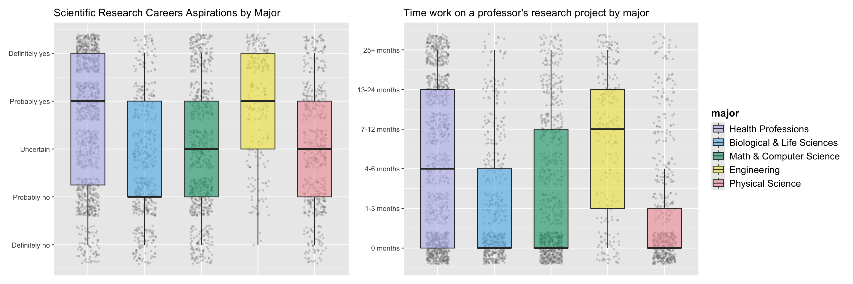

#ggsave("p0.png", combined_plot, width = 15, height = 5, dpi = 300)

hpw_vars <- c("HPW17", "HPW29", "HPW28", "HPW09", "HPW04", 
              "HPW24", "HPW06", "HPW27", "HPW02")
hpw_labels <- c(
  "HPW17" = "Studying/homework",
  "HPW29" = "Studying with other students",
  "HPW28" = "Socializing with friends in person",
  "HPW09" = "Using social media",
  "HPW04" = "Participating in student clubs/groups",
  "HPW24" = "Watching TV/online video content",
  "HPW06" = "Exercising/sports",
  "HPW27" = "Working (for pay) on campus",
  "HPW02" = "Career planning (job searches, networking, etc.)"
)

plot_list <- list()

for (i in seq_along(hpw_vars)) {
  var_name <- hpw_vars[i]
  show_y_axis <- i %in% c(1, 4, 7)
  is_last_plot <- i == 9
  
  plot_list[[i]] <- ggplot(dt, aes(x = major, y = as.numeric(.data[[var_name]]), fill = major)) +
    geom_jitter(width = 0.2, alpha = 0.3, size = 1, color = "gray45", shape = 16) +
    geom_boxplot(alpha = 0.6, outlier.shape = NA, width = 0.6) +
    scale_fill_manual(values = major_colors) +
    scale_y_continuous(
      breaks = 1:8,
      labels = if(show_y_axis) c("None", "<1 hr", "1-2 hrs", "3-5 hrs", "6-10 hrs", 
                                  "11-15 hrs", "16-20 hrs", ">20 hrs") else NULL,
      limits = c(1, 8)) +
    labs(title = hpw_labels[var_name], y = NULL, x = NULL) +
    theme_minimal() +
    theme(
      axis.text.x = element_blank(),  
      axis.ticks.x = element_blank(), 
      axis.text.y = if(show_y_axis) element_text(size = 12) else element_blank(),
      axis.ticks.y = if(show_y_axis) element_line() else element_blank(),
      legend.position = if(is_last_plot) "right" else "none",
      plot.title = element_text(size = 15, face = "bold")
    )
}

combined_hpw_plot <- wrap_plots(plot_list, ncol = 3) +
  plot_layout(guides = "collect") +
  plot_annotation(
    title = "Hours Per Week Spent on Activities by Major",
    theme = theme(plot.title = element_text(size = 20, face = "bold", hjust = 0.5))
  )

print(combined_hpw_plot)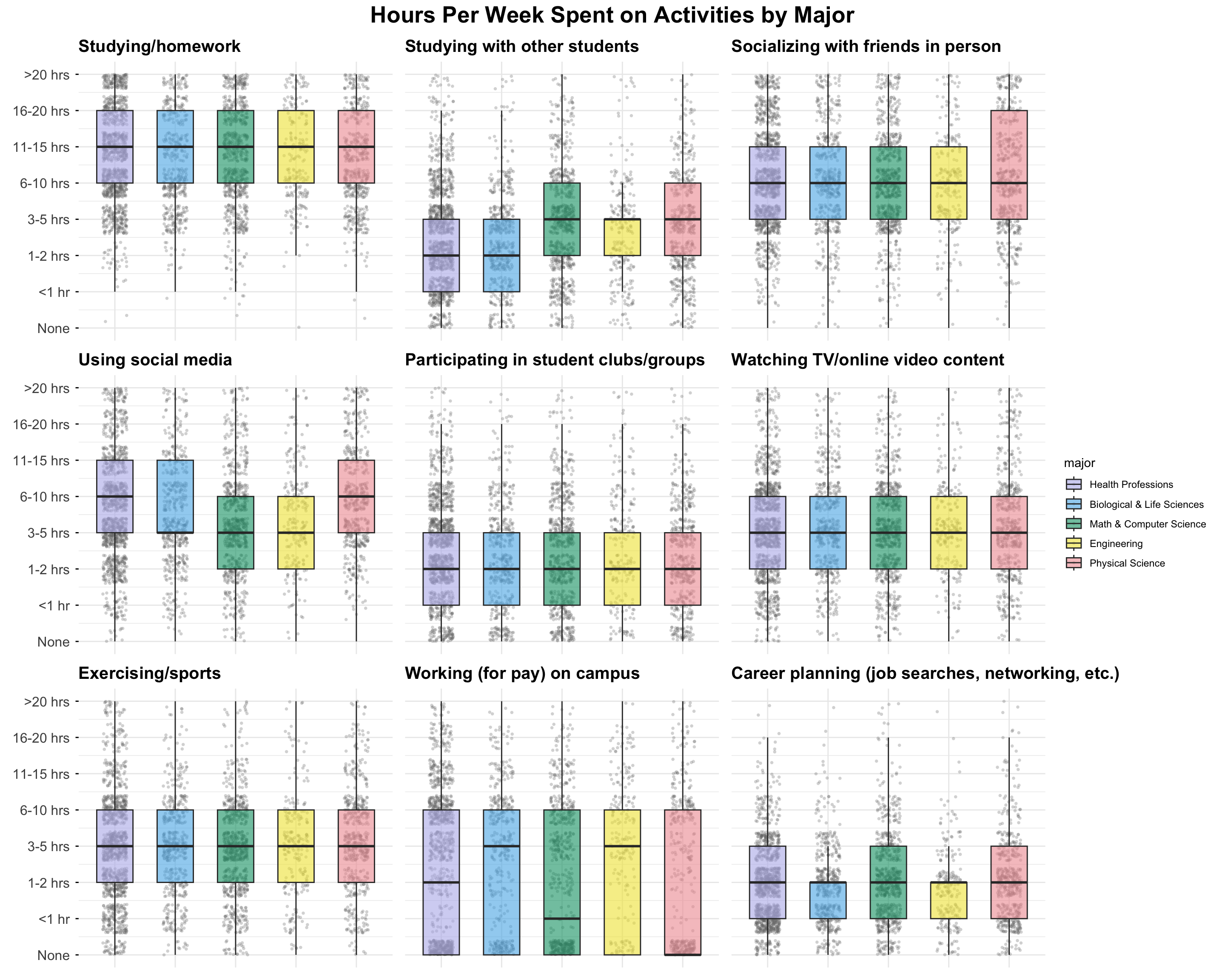

#ggsave("p1.png", combined_hpw_plot, width = 15, height = 10, dpi = 300)

linear regression and qq-plot

dt <- dt %>% mutate(major = relevel(major, ref = "Biological & Life Sciences"))
lm1 <- lm(SCICAREER ~ SCIENCE_SELF_EFFICACY_z + SCIENCE_IDENTITY_z + ACADEMIC_SELFCONCEPT_z +  HABITS_OF_MIND_z +
         MAJORGPA + GOAL19 + GOAL11 + GOAL04 + RESEARCH + 
         HPW17 + HPW29 + HPW28 + HPW09 + HPW04 + HPW24 + HPW06 + HPW27 + HPW02, data = dt)
summary(lm1)

Call:
lm(formula = SCICAREER ~ SCIENCE_SELF_EFFICACY_z + SCIENCE_IDENTITY_z + 
    ACADEMIC_SELFCONCEPT_z + HABITS_OF_MIND_z + MAJORGPA + GOAL19 + 
    GOAL11 + GOAL04 + RESEARCH + HPW17 + HPW29 + HPW28 + HPW09 + 
    HPW04 + HPW24 + HPW06 + HPW27 + HPW02, data = dt)

Residuals:
    Min      1Q  Median      3Q     Max 
-3.6574 -0.7194  0.0327  0.7256  3.5067 

Coefficients:
                         Estimate Std. Error t value Pr(>|t|)    
(Intercept)              2.349907   0.166396  14.122  < 2e-16 ***
SCIENCE_SELF_EFFICACY_z  0.034941   0.029036   1.203 0.228918    
SCIENCE_IDENTITY_z       0.615498   0.031524  19.525  < 2e-16 ***
ACADEMIC_SELFCONCEPT_z  -0.111186   0.021939  -5.068 4.24e-07 ***
HABITS_OF_MIND_z        -0.015615   0.022184  -0.704 0.481560    
MAJORGPA                -0.020372   0.013711  -1.486 0.137426    
GOAL19                   0.370008   0.023275  15.897  < 2e-16 ***
GOAL11                  -0.116779   0.025407  -4.596 4.46e-06 ***
GOAL04                  -0.016020   0.023856  -0.672 0.501924    
RESEARCH                 0.071731   0.011264   6.368 2.17e-10 ***
HPW17                    0.037257   0.014299   2.606 0.009213 ** 
HPW29                   -0.003509   0.013585  -0.258 0.796212    
HPW28                   -0.048605   0.013415  -3.623 0.000295 ***
HPW09                   -0.009554   0.013053  -0.732 0.464264    
HPW04                   -0.019121   0.012025  -1.590 0.111905    
HPW24                    0.009542   0.013153   0.725 0.468241    
HPW06                    0.012262   0.011942   1.027 0.304601    
HPW27                    0.004713   0.008866   0.532 0.595070    
HPW02                    0.006295   0.015441   0.408 0.683532    
---
Signif. codes:  0 '***' 0.001 '**' 0.01 '*' 0.05 '.' 0.1 ' ' 1

Residual standard error: 1.055 on 3327 degrees of freedom
Multiple R-squared:  0.3644,    Adjusted R-squared:  0.361 
F-statistic:   106 on 18 and 3327 DF,  p-value: < 2.2e-16

tidy_lm1 <- tidy(lm1, conf.int = TRUE)
print(tidy_lm1)

# A tibble: 19 × 7
   term                 estimate std.error statistic  p.value conf.low conf.high
   <chr>                   <dbl>     <dbl>     <dbl>    <dbl>    <dbl>     <dbl>
 1 (Intercept)           2.35      0.166      14.1   5.04e-44  2.02      2.68   
 2 SCIENCE_SELF_EFFICA…  0.0349    0.0290      1.20  2.29e- 1 -0.0220    0.0919 
 3 SCIENCE_IDENTITY_z    0.615     0.0315     19.5   1.84e-80  0.554     0.677  
 4 ACADEMIC_SELFCONCEP… -0.111     0.0219     -5.07  4.24e- 7 -0.154    -0.0682 
 5 HABITS_OF_MIND_z     -0.0156    0.0222     -0.704 4.82e- 1 -0.0591    0.0279 
 6 MAJORGPA             -0.0204    0.0137     -1.49  1.37e- 1 -0.0473    0.00651
 7 GOAL19                0.370     0.0233     15.9   6.64e-55  0.324     0.416  
 8 GOAL11               -0.117     0.0254     -4.60  4.46e- 6 -0.167    -0.0670 
 9 GOAL04               -0.0160    0.0239     -0.672 5.02e- 1 -0.0628    0.0308 
10 RESEARCH              0.0717    0.0113      6.37  2.17e-10  0.0496    0.0938 
11 HPW17                 0.0373    0.0143      2.61  9.21e- 3  0.00922   0.0653 
12 HPW29                -0.00351   0.0136     -0.258 7.96e- 1 -0.0301    0.0231 
13 HPW28                -0.0486    0.0134     -3.62  2.95e- 4 -0.0749   -0.0223 
14 HPW09                -0.00955   0.0131     -0.732 4.64e- 1 -0.0351    0.0160 
15 HPW04                -0.0191    0.0120     -1.59  1.12e- 1 -0.0427    0.00446
16 HPW24                 0.00954   0.0132      0.725 4.68e- 1 -0.0162    0.0353 
17 HPW06                 0.0123    0.0119      1.03  3.05e- 1 -0.0112    0.0357 
18 HPW27                 0.00471   0.00887     0.532 5.95e- 1 -0.0127    0.0221 
19 HPW02                 0.00629   0.0154      0.408 6.84e- 1 -0.0240    0.0366 

library(lm.beta)
summary(lm.beta(lm1))

Call:
lm(formula = SCICAREER ~ SCIENCE_SELF_EFFICACY_z + SCIENCE_IDENTITY_z + 
    ACADEMIC_SELFCONCEPT_z + HABITS_OF_MIND_z + MAJORGPA + GOAL19 + 
    GOAL11 + GOAL04 + RESEARCH + HPW17 + HPW29 + HPW28 + HPW09 + 
    HPW04 + HPW24 + HPW06 + HPW27 + HPW02, data = dt)

Residuals:
    Min      1Q  Median      3Q     Max 
-3.6574 -0.7194  0.0327  0.7256  3.5067 

Coefficients:
                         Estimate Standardized Std. Error t value Pr(>|t|)    
(Intercept)              2.349907           NA   0.166396  14.122  < 2e-16 ***
SCIENCE_SELF_EFFICACY_z  0.034941     0.021417   0.029036   1.203 0.228918    
SCIENCE_IDENTITY_z       0.615498     0.365636   0.031524  19.525  < 2e-16 ***
ACADEMIC_SELFCONCEPT_z  -0.111186    -0.084548   0.021939  -5.068 4.24e-07 ***
HABITS_OF_MIND_z        -0.015615    -0.011415   0.022184  -0.704 0.481560    
MAJORGPA                -0.020372    -0.023502   0.013711  -1.486 0.137426    
GOAL19                   0.370008     0.276986   0.023275  15.897  < 2e-16 ***
GOAL11                  -0.116779    -0.066788   0.025407  -4.596 4.46e-06 ***
GOAL04                  -0.016020    -0.010374   0.023856  -0.672 0.501924    
RESEARCH                 0.071731     0.099129   0.011264   6.368 2.17e-10 ***
HPW17                    0.037257     0.041155   0.014299   2.606 0.009213 ** 
HPW29                   -0.003509    -0.004186   0.013585  -0.258 0.796212    
HPW28                   -0.048605    -0.057289   0.013415  -3.623 0.000295 ***
HPW09                   -0.009554    -0.011604   0.013053  -0.732 0.464264    
HPW04                   -0.019121    -0.023976   0.012025  -1.590 0.111905    
HPW24                    0.009542     0.011069   0.013153   0.725 0.468241    
HPW06                    0.012262     0.014947   0.011942   1.027 0.304601    
HPW27                    0.004713     0.007723   0.008866   0.532 0.595070    
HPW02                    0.006295     0.005975   0.015441   0.408 0.683532    
---
Signif. codes:  0 '***' 0.001 '**' 0.01 '*' 0.05 '.' 0.1 ' ' 1

Residual standard error: 1.055 on 3327 degrees of freedom
Multiple R-squared:  0.3644,    Adjusted R-squared:  0.361 
F-statistic:   106 on 18 and 3327 DF,  p-value: < 2.2e-16

par(mfrow = c(2,2))
plot(lm1)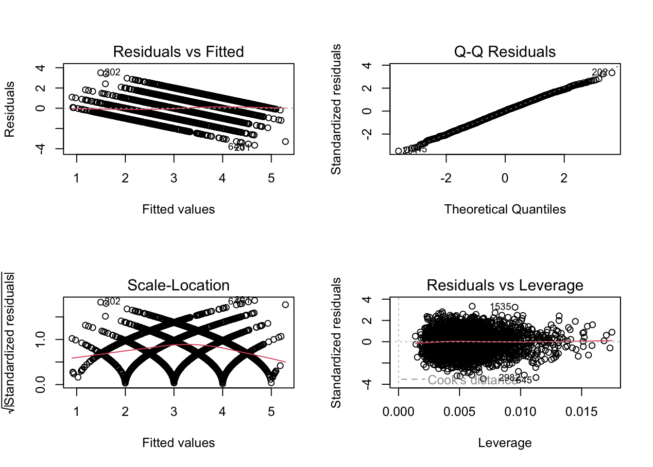

par(mfrow = c(1,1))

2. Univariate Kernel Density Plot

With C

library(Rcpp)

cppFunction('
  NumericVector kde_cpp(NumericVector x, NumericVector eval_points, double bandwidth) {
    int n = x.size();
    int m = eval_points.size();
    NumericVector density(m);
    
    for (int j = 0; j < m; j++) {
      double sum = 0.0;
      for (int i = 0; i < n; i++) {
        double u = (eval_points[j] - x[i]) / bandwidth;
        sum += exp(-0.5 * u * u) / sqrt(2.0 * M_PI);  // Gaussian kernel
      }
      density[j] = sum / (n * bandwidth);
    }
    
    return density;
  }
')

cppFunction('
  NumericMatrix kde_bootstrap_cpp(NumericVector x, NumericVector eval_points, 
                                  double bandwidth, int n_boot) {
    int n = x.size();
    int m = eval_points.size();
    NumericMatrix boot_densities(n_boot, m);
    
    for (int b = 0; b < n_boot; b++) {
     
      NumericVector boot_sample(n);
      for (int i = 0; i < n; i++) {
        int idx = floor(R::runif(0, n));
        boot_sample[i] = x[idx];
      }
      

      for (int j = 0; j < m; j++) {
        double sum = 0.0;
        for (int i = 0; i < n; i++) {
          double u = (eval_points[j] - boot_sample[i]) / bandwidth;
          sum += exp(-0.5 * u * u) / sqrt(2.0 * M_PI);
        }
        boot_densities(b, j) = sum / (n * bandwidth);
      }
    }
    
    return boot_densities;
  }
')

#KDE estimation
kde_estimate_cpp <- function(data, var_name, n_boot = 1000, alpha = 0.05, n_grid = 512) {
  data_clean <- data[[var_name]][!is.na(data[[var_name]])]
  n <- length(data_clean)
  bw_scott <- bw.nrd0(data_clean)
  x_range <- range(data_clean)
  x_padding <- 0.1 * diff(x_range)
  x_grid <- seq(x_range[1] - x_padding, x_range[2] + x_padding, length.out = n_grid)
  #compute original density using Rcpp
  cat(paste0("Computing KDE for ", var_name, "...\n"))
  dens_original <- kde_cpp(data_clean, x_grid, bw_scott)
  #bootstrap for confidence intervals using Rcpp
  cat(paste0("Bootstrapping (", n_boot, " iterations)...\n"))
  boot_densities <- kde_bootstrap_cpp(data_clean, x_grid, bw_scott, n_boot)

  ci_lower <- apply(boot_densities, 2, quantile, probs = alpha/2, na.rm = TRUE)
  ci_upper <- apply(boot_densities, 2, quantile, probs = 1 - alpha/2, na.rm = TRUE)
  
  list(x_grid = x_grid, density = dens_original,ci_lower = ci_lower, ci_upper = ci_upper,
    data_clean = data_clean, bandwidth = bw_scott
  )
}

kde_plot <- function(kde_result, var_label, x_breaks = NULL, x_labels = NULL, 
                     show_y_axis = TRUE) {
  
  dens_df <- data.frame(x = kde_result$x_grid, y = kde_result$density,
    ci_lower = kde_result$ci_lower, ci_upper = kde_result$ci_upper)
  
  p <- ggplot() +
    geom_histogram(data = data.frame(x = kde_result$data_clean), aes(x = x, y = after_stat(density)), 
                   bins = 30, fill = "lightblue", color = "white", alpha = 0.7) +
    geom_ribbon(data = dens_df, aes(x = x, ymin = ci_lower, ymax = ci_upper), fill = "red", alpha = 0.4) +
    geom_line(data = dens_df, aes(x = x, y = y), color = "navy", size = 0.7) +
    labs(title = paste("Distribution of", var_label), x = var_label, y = if(show_y_axis) "Density" else NULL) +
    theme_minimal() +
    theme(plot.title = element_text(size = 11, face = "bold"),
          axis.text.x = element_text(size = 9),
          axis.text.y = if(show_y_axis) element_text(size = 9) else element_blank(),
          axis.ticks.y = if(show_y_axis) element_line() else element_blank(),
          axis.title.y = if(show_y_axis) element_text(size = 10) else element_blank())
  
  if (!is.null(x_breaks) && !is.null(x_labels)) {
    p <- p + scale_x_continuous(breaks = x_breaks, labels = x_labels)
  }
  return(p)
}

#convenience function combining estimation and plotting
kde_ci_cpp <- function(data, var_name, var_label, x_breaks = NULL, x_labels = NULL,
                       n_boot = 1000, alpha = 0.05, 
                       show_y_axis = TRUE, n_grid = 512) {

  kde_result <- kde_estimate_cpp(data, var_name, n_boot, alpha, n_grid)
  p <- kde_plot(kde_result, var_label, x_breaks, x_labels, show_y_axis)
  return(p)
}

p1 <- kde_ci_cpp(dt, "SCIENCE_SELF_EFFICACY_z", "Science Self-Efficacy", n_boot = 1000, show_y_axis = TRUE)

Computing KDE for SCIENCE_SELF_EFFICACY_z...
Bootstrapping (1000 iterations)...

p2 <- kde_ci_cpp(dt, "SCIENCE_IDENTITY_z", "Science Identity", n_boot = 1000, show_y_axis = FALSE)

Computing KDE for SCIENCE_IDENTITY_z...
Bootstrapping (1000 iterations)...

p3 <- kde_ci_cpp(dt, "ACADEMIC_SELFCONCEPT_z", "Academic Self-Concept", n_boot = 1000, show_y_axis = TRUE)

Computing KDE for ACADEMIC_SELFCONCEPT_z...
Bootstrapping (1000 iterations)...

p4 <- kde_ci_cpp(dt, "HABITS_OF_MIND_z", "Habits of Mind", n_boot = 1000, show_y_axis = FALSE)

Computing KDE for HABITS_OF_MIND_z...
Bootstrapping (1000 iterations)...

combined_d_plot <- (p1 | p2) / (p3 | p4)
print(combined_d_plot)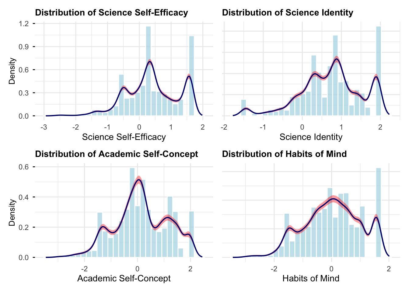

#ggsave("kde_cpp.png", combined_d_plot, width = 10, height = 8, dpi = 300)

without C

#function to create kernel density plot with confidence bounds
kde_ci <- function(data, var_name, var_label, x_breaks = NULL, x_labels = NULL,
                   n_boot = 1000, alpha = 0.05, show_y_axis = TRUE) {
  data_clean <- data[[var_name]][!is.na(data[[var_name]])]
  n <- length(data_clean)
  bw_scott <- bw.nrd0(data_clean)  # Scott's bandwidth
  dens_original <- density(data_clean, bw = bw_scott)
  x_grid <- dens_original$x
  n_grid <- length(x_grid)
  
  #bootstrap to get confidence intervals
  boot_densities <- matrix(NA, nrow = n_boot, ncol = n_grid)
  cat(paste0("Bootstrapping ", var_label, "...\n"))
  for (i in 1:n_boot) {
    #resample with replacement
    boot_sample <- sample(data_clean, size = n, replace = TRUE)
    #calculate density on the same grid
    boot_dens <- density(boot_sample, bw = bw_scott, 
                        from = min(x_grid), to = max(x_grid), n = n_grid)
    boot_densities[i, ] <- boot_dens$y
  }
  
  #calculate confidence intervals (percentile method)
  ci_lower <- apply(boot_densities, 2, quantile, probs = alpha/2, na.rm = TRUE)
  ci_upper <- apply(boot_densities, 2, quantile, probs = 1 - alpha/2, na.rm = TRUE)
  
  
  dens_df <- data.frame(x = x_grid, y = dens_original$y, 
                       ci_lower = ci_lower, ci_upper = ci_upper)
  
  p <- ggplot() +
    geom_histogram(data = data.frame(x = data_clean), 
                   aes(x = x, y = after_stat(density)), 
                   bins = 30, fill = "lightblue", color = "white", alpha = 0.7) +
    geom_ribbon(data = dens_df, aes(x = x, ymin = ci_lower, ymax = ci_upper), 
                fill = "red", alpha = 0.4) +
    geom_line(data = dens_df, aes(x = x, y = y), color = "navy", size = 0.7) +
    labs(title = paste("Distribution of", var_label), 
         x = var_label, 
         y = if(show_y_axis) "Density" else NULL) +
    theme_minimal() +
    theme(plot.title = element_text(size = 11, face = "bold"),
          axis.text.x = element_text(size = 9),
          axis.text.y = if(show_y_axis) element_text(size = 9) else element_blank(),
          axis.ticks.y = if(show_y_axis) element_line() else element_blank(),
          axis.title.y = if(show_y_axis) element_text(size = 10) else element_blank())
  
  if (!is.null(x_breaks) && !is.null(x_labels)) {
    p <- p + scale_x_continuous(breaks = x_breaks, labels = x_labels)
  }
  
  return(p)
}

#create plots - only left side (p1 and p3) show y-axis
p1 <- kde_ci(dt, "SCIENCE_SELF_EFFICACY_z", "Science Self-Efficacy", n_boot = 1000, show_y_axis = TRUE)

Bootstrapping Science Self-Efficacy...

p2 <- kde_ci(dt, "SCIENCE_IDENTITY_z", "Science Identity", n_boot = 1000, show_y_axis = FALSE)

Bootstrapping Science Identity...

p3 <- kde_ci(dt, "ACADEMIC_SELFCONCEPT_z", "Academic Self-Concept", n_boot = 1000, show_y_axis = TRUE)

Bootstrapping Academic Self-Concept...

p4 <- kde_ci(dt, "HABITS_OF_MIND_z", "Habits of Mind", n_boot = 1000, show_y_axis = FALSE)

Bootstrapping Habits of Mind...

combined_d_plot <- (p1 | p2) / (p3 | p4)
print(combined_d_plot)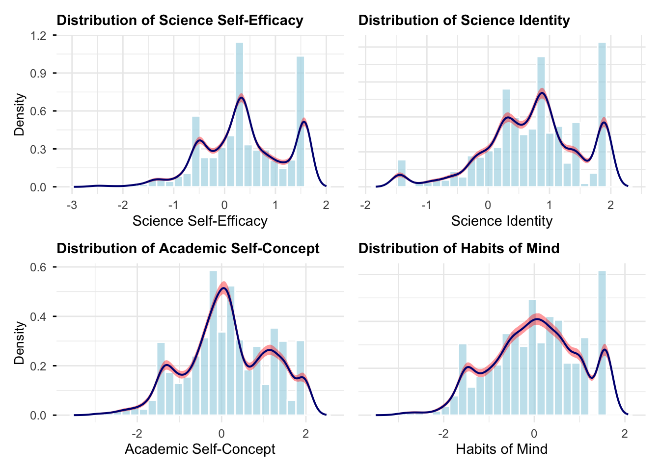

#ggsave("p3.png", combined_d_plot, width = 9, height = 6, dpi = 300)

3. Kernel Regression Esimate

Rcpp::cppFunction("
NumericVector nadaraya_watson(int n, NumericVector X, NumericVector Y, 
                               int m, NumericVector g2, double b) {
  NumericVector res2(m);

  for(int j = 0; j < m; j++) {
    double numerator = 0.0;
    double denominator = 0.0;
  
    for(int i = 0; i < n; i++) {
      // Gaussian kernel: exp(-0.5 * ((x - xi) / b)^2)
      double u = (g2[j] - X[i]) / b;
      double kernel_weight = exp(-0.5 * u * u);
      
      numerator += kernel_weight * Y[i];
      denominator += kernel_weight;
    }
    
    if(denominator > 0) {
      res2[j] = numerator / denominator;
    } else {
      res2[j] = NA_REAL;
    }
  }
  
  return res2;
}
")

run_kernel_reg <- function(X, Y, B = 200) {
  n <- length(X)
  b <- bw.nrd(X)
  m <- 100
  g <- seq(min(X), max(X), length.out = m)
  
  fit <- nadaraya_watson(n, X, Y, m, g, b)
  
  #bootstrap
  boot_mat <- matrix(NA, B, m)
  for(i in 1:B) {
    idx <- sample(n, replace = TRUE)
    boot_mat[i,] <- nadaraya_watson(n, X[idx], Y[idx], m, g, b)
  }
  
  list(X = X, Y = Y, grid = g, fit = fit,
       lower = apply(boot_mat, 2, quantile, 0.025, na.rm = TRUE),
       upper = apply(boot_mat, 2, quantile, 0.975, na.rm = TRUE))
}

reg1 <- run_kernel_reg(dt$RESEARCH, dt$SCIENCE_IDENTITY_z)
reg2 <- run_kernel_reg(dt$RESEARCH, dt$SCIENCE_SELF_EFFICACY_z)
reg3 <- run_kernel_reg(dt$RESEARCH, dt$ACADEMIC_SELFCONCEPT_z)
reg4 <- run_kernel_reg(dt$RESEARCH, dt$HABITS_OF_MIND_z)

par(mfrow = c(2, 2), mar = c(4, 4, 3, 1))

plot_reg <- function(r, xlab, ylab, title) {
  plot(r$X, r$Y, pch = 1, col = "lightblue", main = title, 
       xlab = xlab, ylab = ylab, xaxt = "n")  # xaxt = "n" suppresses default x-axis
  axis(1, at = 1:6, labels = c("0 m", "1-3 m", "4-6 m", "7-12 m", "13-24 m", "25+ m"))  
  lines(r$grid, r$fit, col = "blue", lwd = 2)
  lines(r$grid, r$lower, col = "red", lty = 2)
  lines(r$grid, r$upper, col = "red", lty = 2)
}

#png("p6_base.png", width = 9, height = 7, units = "in", res = 300)
par(mfrow = c(2, 2), mar = c(4, 4, 3, 1))
plot_reg(reg1, "Undergraduate Research Time", "Science Identity", "Research - Science Identity")
plot_reg(reg2, "Undergraduate Research Time", "Academic Self-Concept", "Research - Science Self-efficacy")
plot_reg(reg3, "Undergraduate Research Time", "Academic Self-Concept", "Research - Academic Self-Concept")
plot_reg(reg4, "Undergraduate Research Time", "Science Identity", "Research - Habits of Mind")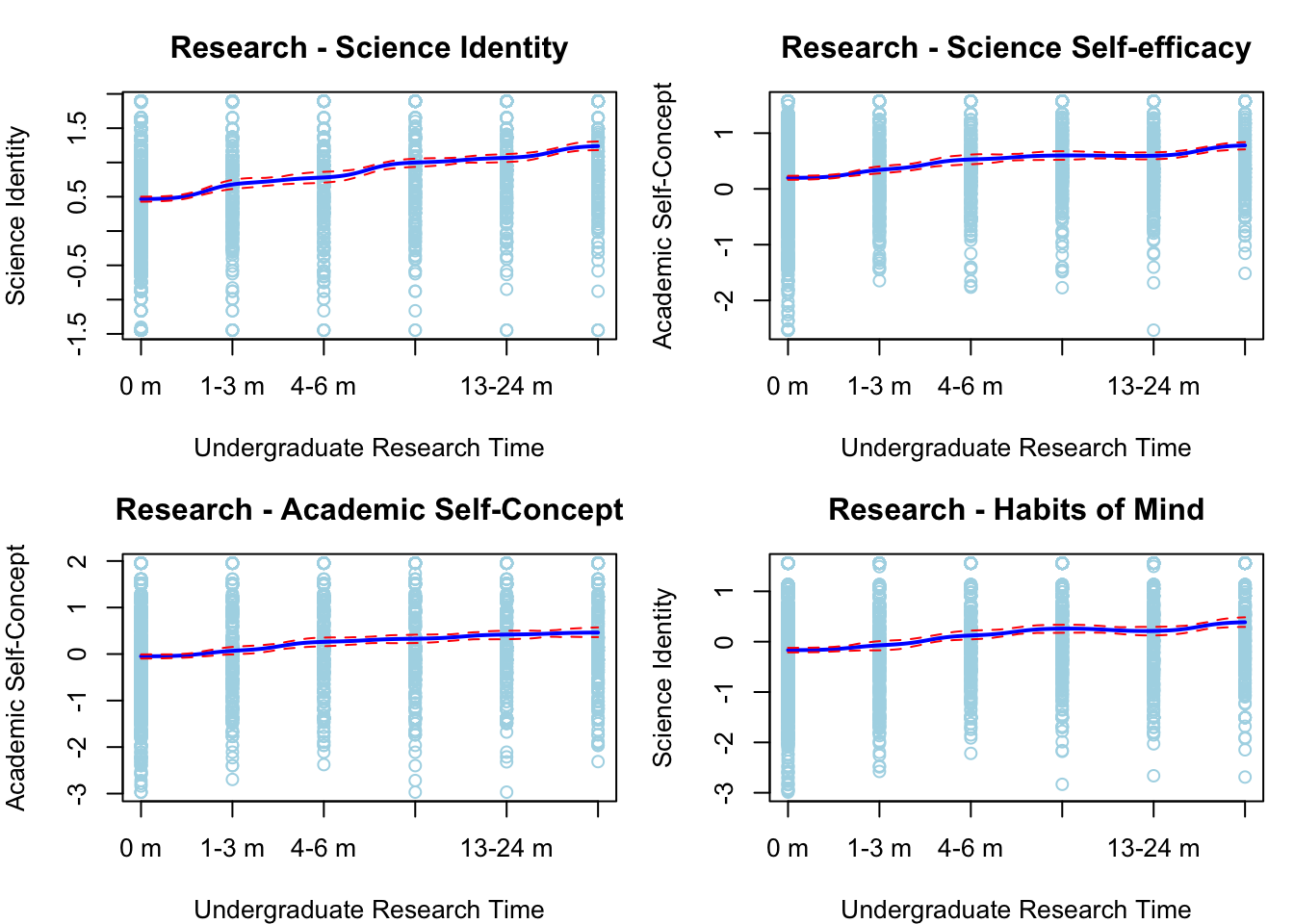

#dev.off()

4. Prediction using ML algorithms

• Create a binary varible for science career plan (1 = yes (4=Probably yes; 5=Definitely yes), 0 = No)
• Use 10 folds cross-validation , have training set and test set
• Use ML algriothm like trees, knn, logistic regression, and other to predict whether students will pursue a science career
• Report model accuracy, auc roc plots.
• check variable importance

library(caret)
library(pROC)
library(rpart) #recursive patitioning and regression trees
library(rpart.plot) #visualization for rpart decision trees
library(randomForest)
library(xgboost)
library(glmnet)

dt <- dt %>% mutate(SCICAREER_binary = ifelse(as.numeric(as.character(SCICAREER)) >= 4, 1, 0))

model_vars <- c("SCICAREER_binary", "SCIENCE_SELF_EFFICACY", "SCIENCE_IDENTITY", "ACADEMIC_SELFCONCEPT",
                "HABITS_OF_MIND", "MAJORGPA", "GOAL19", "GOAL11", "GOAL04", "RESEARCH",
                "HPW17", "HPW29", "HPW28", "HPW09", "HPW04", "HPW24", "HPW06", "HPW27", "HPW02")

dt_model <- dt %>% select(all_of(model_vars)) %>% drop_na() %>%
  mutate(SCICAREER_binary = factor(SCICAREER_binary, levels = c(0, 1), labels = c("No", "Yes")))

for(var in model_vars[-1]) {
  dt_model[[var]] <- as.numeric(as.character(dt_model[[var]]))
}

#set up 10-folds cross-validation
set.seed(612)
train_control <- trainControl(method = "cv", number = 10, savePredictions = "final",
                              classProbs = TRUE, summaryFunction = twoClassSummary)

#model 1: logistic regressin
m_logit <- train(SCICAREER_binary ~ ., data = dt_model, method = "glm",
  family = "binomial", trControl = train_control, metric = "ROC")

#model 2: decision tree
m_tree <- train(SCICAREER_binary ~ ., data = dt_model, method = "rpart",
  trControl = train_control, metric = "ROC", tuneLength = 10)

#model 3: random forest
m_rf <- train(SCICAREER_binary ~ ., data = dt_model, method = "rf", trControl = train_control,
  metric = "ROC", tuneLength = 5, importance = TRUE)

#model 4: KNN
m_knn <- train(SCICAREER_binary ~ ., data = dt_model,method = "knn", trControl = train_control,
  metric = "ROC", preProcess = c("center", "scale"), tuneLength = 10)

#model 5: Gradient Boosting (XGBoost)
m_xgb <- train(SCICAREER_binary ~ ., data = dt_model, method = "xgbTree", trControl = train_control,
  metric = "ROC", tuneLength = 3, verbosity = 0)


results <- resamples(list(Logistic = m_logit, Tree = m_tree, RandomForest = m_rf,
            KNN = m_knn, XGBoost = m_xgb))
summary(results)

Call:
summary.resamples(object = results)

Models: Logistic, Tree, RandomForest, KNN, XGBoost 
Number of resamples: 10 

ROC 
                  Min.   1st Qu.    Median      Mean   3rd Qu.      Max. NA's
Logistic     0.7538151 0.7990175 0.8101776 0.8077944 0.8201123 0.8430392    0
Tree         0.7382846 0.7542069 0.7657015 0.7709614 0.7864987 0.8127519    0
RandomForest 0.7876452 0.8013756 0.8057399 0.8038253 0.8091662 0.8154019    0
KNN          0.7493034 0.7534711 0.7659354 0.7746876 0.7923890 0.8233336    0
XGBoost      0.7884052 0.7934693 0.8163744 0.8104399 0.8239514 0.8302260    0

Sens 
                  Min.   1st Qu.    Median      Mean   3rd Qu.      Max. NA's
Logistic     0.7445652 0.7759563 0.7771739 0.7805179 0.7986383 0.8097826    0
Tree         0.6739130 0.7431694 0.7520492 0.7527322 0.7785326 0.8206522    0
RandomForest 0.7500000 0.7744565 0.7868852 0.7854241 0.7967302 0.8260870    0
KNN          0.7650273 0.7855191 0.8043478 0.8038994 0.8206522 0.8478261    0
XGBoost      0.7336957 0.7486339 0.7738477 0.7696098 0.7894022 0.7989130    0

Spec 
                  Min.   1st Qu.    Median      Mean   3rd Qu.      Max. NA's
Logistic     0.6357616 0.6506623 0.6622517 0.6781457 0.7036424 0.7549669    0
Tree         0.6225166 0.6539735 0.6821192 0.6741722 0.6887417 0.7152318    0
RandomForest 0.6291391 0.6456954 0.6655629 0.6655629 0.6837748 0.7086093    0
KNN          0.5496689 0.5596026 0.5695364 0.5913907 0.6142384 0.6688742    0
XGBoost      0.6357616 0.6771523 0.7052980 0.7039735 0.7334437 0.7549669    0

perf_p1 <- bwplot(results, metric = "ROC", main = "ROC AUC across 10 Folds")
perf_p2 <- bwplot(results, metric = "Sens", main = "Sensitivity across 10 Folds")
perf_p3 <- bwplot(results, metric = "Spec", main = "Specificity across 10 Folds")

combined_perf <- grid.arrange(perf_p1, perf_p2, perf_p3, ncol = 3)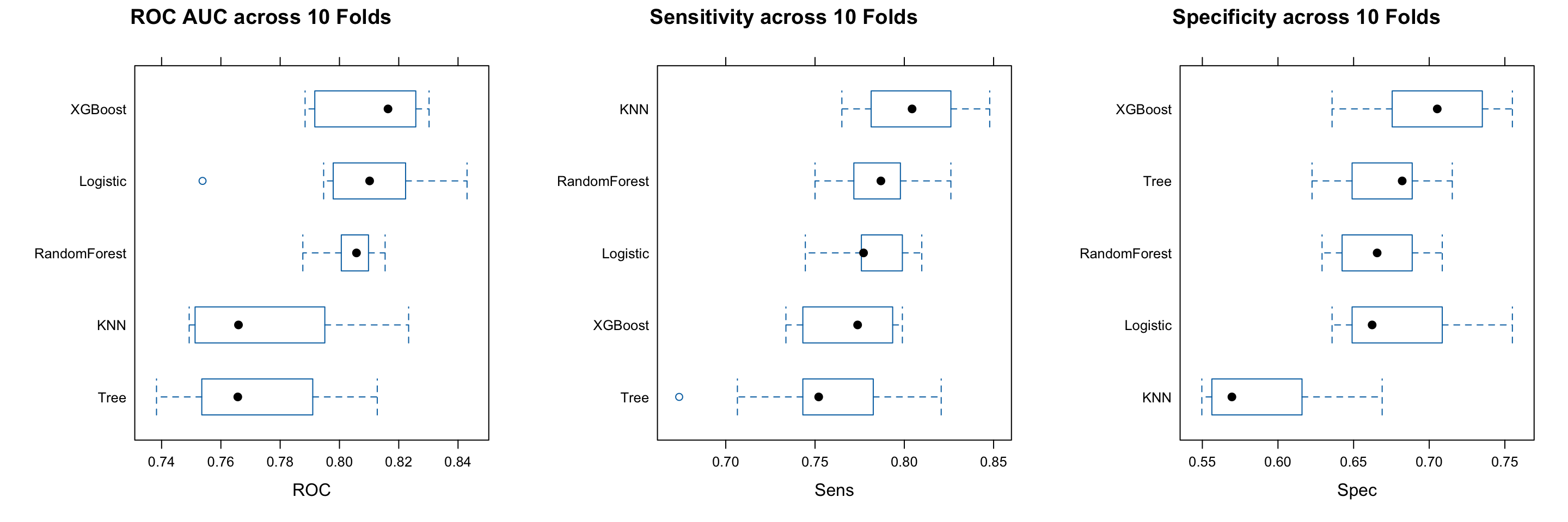

#ggsave("p4.png", combined_perf, width = 15, height = 5, dpi = 300, bg = "white")

check variables importance

Most caret::varImp() outputs are scaled by default: Take the most important predictor; Assign it a value of 100; Scale all other predictors proportionally between 0 and 100.

#extract importance from all models
get_importance <- function(model, model_name) {
  tryCatch({
    imp <- varImp(model, scale = TRUE)
    data.frame(Variable = rownames(imp$importance), Importance = imp$importance[, 1], Model = model_name)
  }, error = function(e) {
    return(NULL)
  })
}

logit_imp <- get_importance(m_logit, "Logistic")
tree_imp <- get_importance(m_tree, "Tree")
rf_imp <- get_importance(m_rf, "RandomForest")
xgb_imp <- get_importance(m_xgb, "XGBoost")

#combine all (excluding KNN since it doesn't provide meaningful importance)
all_imp <- bind_rows(logit_imp, tree_imp, rf_imp, xgb_imp)

top10_vars <- all_imp %>% group_by(Variable) %>%
  summarise(Avg_Importance = mean(Importance, na.rm = TRUE)) %>%
  arrange(desc(Avg_Importance)) %>%
  head(10) %>% pull(Variable)

plot_data <- all_imp %>% filter(Variable %in% top10_vars)

#comparison plot
p <- ggplot(plot_data,aes(x = reorder(Variable, Importance), y = Importance, fill = Model)) +
  geom_col(position = "dodge", alpha = 0.8) +
  coord_flip() + 
  scale_fill_brewer(palette = "Set2") +
  labs(title = "Top 10 Predictors Across 4 Models (Logistic, Tree, RF, XGBoost)",  x = NULL, y = "Importance (0-100)") +
  theme_minimal() +
  theme(plot.title = element_text(face = "bold", size = 11), 
        legend.position = "top")

print(p)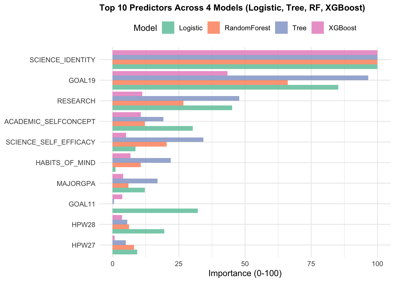

#ggsave("p5.png", p, width = 10, height = 6, dpi = 300)

summary_table <- all_imp %>%
  filter(Variable %in% top10_vars) %>%
  tidyr::pivot_wider(names_from = Model, values_from = Importance) %>%
  mutate(Average = rowMeans(select(., -Variable), na.rm = TRUE)) %>%
  arrange(desc(Average))

print(summary_table)

# A tibble: 10 × 6
   Variable              Logistic    Tree RandomForest XGBoost Average
   <chr>                    <dbl>   <dbl>        <dbl>   <dbl>   <dbl>
 1 SCIENCE_IDENTITY        100    100           100    100      100   
 2 GOAL19                   85.2   96.6          66.1   43.4     72.8 
 3 RESEARCH                 45.1   47.8          26.7   11.2     32.7 
 4 ACADEMIC_SELFCONCEPT     30.2   19.2          12.2   10.6     18.1 
 5 SCIENCE_SELF_EFFICACY     8.63  34.3          20.4    5.04    17.1 
 6 HABITS_OF_MIND            1.08  22.0          10.7    6.75    10.1 
 7 MAJORGPA                 12.2   16.9           5.95   4.03     9.79
 8 GOAL11                   32.2    0.550         0      3.64     9.09
 9 HPW28                    19.5    5.51          6.18   3.50     8.68
10 HPW27                     9.28   4.95          8.09   0.779    5.78