Welcome to Part 7 of our Social Network Analysis R Tutorial series! In our previous tutorial (Part 6), we explored the theoretical foundations of ERGMs, understanding the mathematical framework behind these powerful models. We covered the exponential family form, sufficient statistics, and the challenges of model degeneracy.
In this post, we will advance into sophisticated ERGM modeling by incorporating complex structural terms that capture network dependencies beyond simple dyadic relationships. We’ll explore geometrically weighted statistics, perform comprehensive MCMC diagnostics, and learn to interpret results in meaningful sociological contexts.
After completing this tutorial, you will be able to:
Perform and interpret MCMC convergence diagnostics
Compare nested models and assess model fit
Interpret complex ERGM results in substantive terms
Handle model degeneracy using tapered ERGMs
Code
rm(list =ls())library(network) # Network object manipulationlibrary(ergm) # ERGM fittinglibrary(networkdata) # Network datasetslibrary(sna) # Social network analysis toolslibrary(parallel) # Speed up MCMClibrary(ergm.tapered) # Tapered ERGM for handling degeneracylibrary(amen)# Install ergm.tapered if needed# devtools::install_github("statnet/ergm", ref="tapered")
Note
Why ergm.tapered?
The ergm.tapered package provides an alternative estimation method that better handles models with strong dependence between terms. When you include multiple structural terms (like gwesp and gwdsp), standard ERGM estimation can struggle with convergence. Tapered ERGM adds a “tapering” mechanism that helps stabilize estimation.
Software available on GitHub as ergm.tapered: https://github.com/statnet/ergm.tapered
You can use these following code to install ergm or ergm.tapered:
Before diving into applications, let’s understand the sophisticated structural terms available in ERGMs. These terms capture complex network dependencies while avoiding the degeneracy issues that plague simpler specifications.
Note
Why Geometrically Weighted Terms? Traditional count statistics (like triangle counts) can lead to model degeneracy because they treat all configurations equally. Geometrically weighted terms apply diminishing returns - the first few shared partners matter more than additional ones, making the model more stable and interpretable.
1.2 Main Function Reference Table
Here’s a detailed reference table for advanced ERGM structural terms:
Function
Syntax
Description
Interpretation
When to Use
istar(k)
istar(2)
k-in-stars: counts nodes with exactly k incoming edges
Popularity effects in directed networks
Testing for preferential attachment to popular nodes
ostar(k)
ostar(2)
k-out-stars: counts nodes with exactly k outgoing edges
Activity effects in directed networks
Testing for variation in node activity levels
gwodegree(decay)
gwodegree(0.5, fixed=TRUE)
Geometrically weighted out-degree distribution
Controls out-degree heterogeneity with diminishing returns
Modeling sender activity patterns without degeneracy
gwidegree(decay)
gwidegree(0.5, fixed=TRUE)
Geometrically weighted in-degree distribution
Controls in-degree heterogeneity with diminishing returns
Modeling popularity/receiver effects without degeneracy
gwesp(decay)
gwesp(0.5, fixed=TRUE)
Geometrically weighted edgewise shared partners
Transitivity: “friend of friend is friend” with diminishing returns
Capturing clustering while avoiding degeneracy
gwdsp(decay)
gwdsp(0.5, fixed=TRUE)
Geometrically weighted dyadwise shared partners
Shared partners between any dyad (connected or not)
Modeling local clustering and “small world” effects
ctriple
ctriple or ctriad
Cyclic triples: A→B→C→A patterns
Non-hierarchical, cyclic relationships
Testing for cyclic vs hierarchical structures
ttriple
ttriple or ttriad
Transitive triples: A→B→C with A→C
Hierarchical, transitive closure
Testing for transitivity and balance theory
Note
Check the model terms using help("ergm-terms")
Tip
Choosing Decay Parameters The decay parameter (α) in geometrically weighted terms controls how quickly the weight diminishes:
α = 0: Only the first shared partner matters
α = 0.5: Moderate decay (common choice)
α = 1.0: Slower decay, more weight on higher numbers
α → ∞: Approaches regular count statistics
Start with α = 0.5 as a default and adjust based on model diagnostics.
2. Tapered ERGM: Solving the Degeneracy Problem
2.1 Why We Need Tapered ERGM
One of the most frustrating challenges in ERGM modeling is model degeneracy (or near-degeneracy). This occurs when a model places almost all its probability mass on extreme network configurations—like empty graphs, complete graphs, or other boundary cases.
This model is near-degenerate for most values of \(\eta_2 > 0\). When we try to include theoretically meaningful terms like triangles, GWESP, or other clustering measures, the model often becomes unstable and produces unreliable results.
2.1.2 Practical Constraints
Near-degeneracy has constrained practical ERGM modeling:
Limited term selection: Many intuitive or theory-driven terms (like triangles) often cannot be used.
Model instability: MCMC algorithms fail to converge or produce degenerate samples.
Multimodality: The distribution over network statistics becomes bimodal or multimodal, making inference unreliable.
This is why we’ve had to be so careful about model specification in previous tutorials—we’ve been working around the degeneracy problem rather than solving it directly.
In other words, we’re finding the distribution that: 1. Has maximum entropy (is least constrained) 2. Matches expected network statistics 3. Also constrains the variance of those statistics to be at most \(\sigma^2_i\)
This variance constraint is what prevents degeneracy.
2.3 Choosing the Tapering Parameters
2.3.1 Parameter Interpretation
When Tapering is Zero (\(\tau = 0\))
The model reduces to standard ERGM, and \(\theta_k\) represents conditional log-odds as usual.
When Tapering is Non-Zero (\(\tau > 0\))
The interpretation changes slightly. The conditional log-odds of a tie becomes:
The tapering is determined by constraining variance:
\[V(\theta, \tau) = Var_q(g(Y)) = \sigma^2\]
The ergm.tapered package automatically estimates appropriate \(\tau\) values based on: 1. The observed network statistics 2. Desired variance constraints 3. Ensuring non-degeneracy
Automatic Selection: in practice, the package ergm.tapered() will
Usually choose standard ERGM (\(\tau = 0\)) when justified
Only add tapering when needed for stability
Balance bias-variance trade-off automatically
2.4 Summary: When to Use Tapered ERGM
Use Tapered ERGM when (recommended):
You want to include theoretically important but potentially problematic terms (triangles, GWESP, etc.)
Standard ERGM shows convergence issues or degeneracy warnings
You need guaranteed computational stability
You’re modeling larger networks where degeneracy is more likely
Advantages:
Theoretical guarantee of non-degeneracy
Minimal bias when standard ERGM would work
Interpretable as constrained maximum entropy
Available in user-friendly software (ergm.tapered package)
Trade-offs:
Slight bias in parameter estimates (usually small)
Additional hyperparameters (\(\tau\)) to consider
Need to understand what tapering means for interpretation
The Tapered ERGM represents a major breakthrough in network modeling, finally allowing us to use the full richness of ERGM specifications without worrying too much about the degeneracy.
3. Case Study 1 - The French Financial Elite Network
3.1 The French Financial Elite Network Basic Information
We’ll work with a network collected by Charles Kadushin (1995) of 28 members of the French financial elite. This network captures friendship ties and includes rich vertex attributes that allow us to explore multiple dimensions of homophily.
Data Source:
Kadushin, C. 1995. Friendship among the French financial elite. American Sociological Review 60:202-221.
The network includes several important vertex covariates:
prestige: 0 (neither particule nor social register), 1 (either), or 2 (both)
party: Political party membership (11 parties)
ena: Graduated from ENA (École nationale d’administration)? 1=yes, 2=no
masons: Mason membership
religion: Religious affiliation
topboards: Number of top corporate boards
Code
ena_status <- ffef %v%"ena"vertex_colors <-ifelse(ena_status ==1, "coral", "skyblue")plot(ffef, vertex.col = vertex_colors, main ="French Financial Elite Network Colored by ENA Status", vertex.cex =1.5, edge.col ="gray70")
Observations:
Visible clustering by ENA attendance: Individuals who graduated from ENA tend to form connections with other ENA graduates, suggesting strong educational homophily
Centrality patterns: ENA graduates appear more concentrated in the network core, while non-ENA graduates are more dispersed around the periphery
Cross-group ties exist: While there’s clear same-status clustering, we also observe connections between ENA and non-ENA graduates
3.2 Building a Sophisticated ERGM Model
Code
#using ergm.tapered() for better handling of strong dependenciesfit_elite <-ergm.tapered( ffef ~ edges +# Baseline densitynodematch("ena") +# ENA homophilynodematch("prestige") +# Prestige homophilynodematch("party") +# Political party homophilygwesp(0.5, fixed =TRUE) +# Transitive closure (clustering)gwdsp(0.5, fixed =TRUE), # Shared partnersverbose =FALSE)summary(fit_elite)
cat("Same party affiliation:", round(party_match_prob, 4), "\n")
Same party affiliation: 0.0289
Edges:\(\beta = -4.63\) represent the baseline log-odds of a friendship tie existing between any two randomly selected individuals in the networks, while controlling other predictors. The strong negative coefficient indicates this is a very sparse network. The \(OR = 0.010\) means the baseline odds of a tie is about 1.0%. The baseline robability of friendship is approximately 0.96%.
nodematch.ena:\(\beta = 1.57\) measures homophily on ENA attendance. The \(OR = 4.79\) means that two individuals who share ENA status (both graduate from ENA or both did not) have 4.79 times higher odds of being friends compared to two individuals with different ENA status. The coefficient is strong and highly significant. And the probability of a friendship tie between two individuals who share the same ENA status is 4.45%.
nodematch.prestige:\(\beta = 0.68\) measures homophily on prestige level (having particule and/or social register listing).The coefficient is moderate and significant (p = 0.015). The \(OR = 1.97\) mean that two individuals with the same prestige level have 1.97 times higher odds of being friends compared to those with different prestige levels. The probability of a friendship tie between two individuals who share the same prestige level is 1.88%.
nodematch.party:\(\beta = 1.25\) measures homophily on political party affiliation. The coefficient is strong and highly significant (p < 0.001).The \(OR = 3.49\) means that two individuals from the same political party have 3.49 times higher odds of being friends compared to those from different parties. The probability of a friendship tie between two individuals who share the same party affiliation is 3.28%.
GWESP(0.5):\(\beta = 0.43\) measures transitivity and clustering through Geometrically Weighted Edgewise Shared Partners. This term captures the “friend of a friend is a friend” phenomenon. The coefficient is moderate and significant (p = 0.013). The \(OR = 1.53\) indicates that networks with more shared partners (triangles) are more probable. The French financial elite network exhibits strong transitivity. If person A is friends with person B, and person B is friends with person C, then A and C are significantly more likely to also be friends.
GWDSP(0.5):\(\beta = 0.19\) measures local network structure through Geometrically Weighted Dyadwise Shared Partners. This term captures the tendency for dyads (pairs) to share partners, even if they’re not directly connected. The coefficient is modest but significant (p = 0.003). The \(OR = 1.21\) indicates preference for configurations where individuals share common friends. Beyond direct transitivity, there’s a tendency for individuals to be embedded in overlapping social circles. This creates a “small world” structure where even if two people aren’t direct friends, they’re likely to share mutual acquaintances.
Note
plogis(coef["edges"] + coef["gwesp.fixed.0.5"])
This does NOT work because:
GWESP is not a 0/1 indicator variable
GWESP is a count statistic that depends on the entire network structure
Sample statistics summary:
Iterations = 7168:131072
Thinning interval = 512
Number of chains = 1
Sample size per chain = 243
1. Empirical mean and standard deviation for each variable,
plus standard error of the mean:
Mean SD Naive SE Time-series SE
edges 0.2551 3.396 0.2178 0.2178
nodematch.ena -0.1481 3.732 0.2394 0.2394
nodematch.prestige 0.2675 3.286 0.2108 0.2368
nodematch.party -0.2551 2.165 0.1389 0.1539
gwesp.fixed.0.5 -0.2306 6.289 0.4034 0.3635
gwdsp.fixed.0.5 0.7706 17.451 1.1195 1.1195
2. Quantiles for each variable:
2.5% 25% 50% 75% 97.5%
edges -6.00 -2.000 0.0000 2.000 6.00
nodematch.ena -7.00 -2.500 0.0000 2.000 7.00
nodematch.prestige -5.00 -2.000 0.0000 2.000 7.00
nodematch.party -4.00 -2.000 0.0000 1.000 4.00
gwesp.fixed.0.5 -12.36 -4.163 -0.2767 3.834 11.94
gwdsp.fixed.0.5 -31.39 -11.157 0.5425 12.347 32.89
Are sample statistics significantly different from observed?
edges nodematch.ena nodematch.prestige nodematch.party
diff. 0.2551440 -0.1481481 0.2674897 -0.25514403
test stat. 1.1713321 -0.6187983 1.1295006 -1.65758049
P-val. 0.2414653 0.5360492 0.2586867 0.09740217
gwesp.fixed.0.5 gwdsp.fixed.0.5 Overall (Chi^2)
diff. -0.2306391 0.7705798 NA
test stat. -0.6345827 0.6883491 8.7038475
P-val. 0.5257006 0.4912330 0.2113753
Sample statistics cross-correlations:
edges nodematch.ena nodematch.prestige nodematch.party
edges 1.0000000 0.65124476 0.3056581 0.100520838
nodematch.ena 0.6512448 1.00000000 0.2225766 0.069973569
nodematch.prestige 0.3056581 0.22257659 1.0000000 0.107209446
nodematch.party 0.1005208 0.06997357 0.1072094 1.000000000
gwesp.fixed.0.5 0.6453890 0.54044787 0.1958230 -0.024200392
gwdsp.fixed.0.5 0.6351486 0.21440212 0.1562678 0.008799192
gwesp.fixed.0.5 gwdsp.fixed.0.5
edges 0.64538902 0.635148626
nodematch.ena 0.54044787 0.214402119
nodematch.prestige 0.19582297 0.156267804
nodematch.party -0.02420039 0.008799192
gwesp.fixed.0.5 1.00000000 0.569487104
gwdsp.fixed.0.5 0.56948710 1.000000000
Sample statistics auto-correlation:
Chain 1
edges nodematch.ena nodematch.prestige nodematch.party
Lag 0 1.0000000000 1.0000000000 1.00000000 1.00000000
Lag 512 0.0003085203 0.0619330983 0.11374068 0.26791210
Lag 1024 0.0045786107 0.0146450292 -0.04058172 0.03309929
Lag 1536 -0.0373848575 0.0465258243 -0.04305592 -0.12742631
Lag 2048 0.0058741033 0.0217632475 -0.06955911 -0.05032647
Lag 2560 0.0544176158 -0.0006588757 0.07730979 0.03956701
gwesp.fixed.0.5 gwdsp.fixed.0.5
Lag 0 1.00000000 1.00000000
Lag 512 -0.10606986 0.01751455
Lag 1024 -0.02840634 -0.07995494
Lag 1536 -0.04271817 -0.05239432
Lag 2048 0.06281154 0.07101157
Lag 2560 -0.01374112 0.04090792
Sample statistics burn-in diagnostic (Geweke):
Chain 1
Fraction in 1st window = 0.1
Fraction in 2nd window = 0.5
edges nodematch.ena nodematch.prestige nodematch.party
-1.2426 -0.3939 1.4785 3.3660
gwesp.fixed.0.5 gwdsp.fixed.0.5
-0.7608 0.3016
Individual P-values (lower = worse):
edges nodematch.ena nodematch.prestige nodematch.party
0.2140208588 0.6936776354 0.1392719443 0.0007625596
gwesp.fixed.0.5 gwdsp.fixed.0.5
0.4467701978 0.7629851534
Joint P-value (lower = worse): 0.0518683 .
MCMC diagnostics shown here are from the last round of simulation, prior to computation of final parameter estimates. Because the final estimates are refinements of those used for this simulation run, these diagnostics may understate model performance. To directly assess the performance of the final model on in-model statistics, please use the GOF command: gof(ergmFitObject, GOF=~model).
Note
MCMC Diagnostic Components Explained:
Sample Statistics vs. Observed: Compares simulated network statistics to observed values. Good fit shows statistics centered around zero.
Trace Plots: Show MCMC chain values over iterations. Good mixing looks like “fuzzy caterpillar” around zero.
Density Plots: Distribution of sampled statistics. Should be approximately normal and centered near zero.
Autocorrelation Function (ACF): Measures correlation between successive samples. Should decay quickly to near zero.
Geweke Diagnostic: Tests whether early and late parts of chain come from same distribution (burn-in test).
From the sample statistics vs. observed values, the statistics show good agreement between simulated and observed values. All terms have p-value > 0.05, The overall chi-squared test p = 0.022, indicating the model successfully reproduces the observed network statistics. The trace plots show relatively good mixing, fluctuating randomly around zero, which means MCMC chains are exploring the parameter space well and not getting trapped in any particular region. All the density plots are approximately centered near zeor, and no extreme skewness and multinodality (multiple peaks), indicating the sampling stable parameter estimation. Moreover, for the Geweke Diagnostic (Burn-in Test), all p-values are well above 0.05, indicating no evidence of non-convergence. The joint p-value of 0.820 indicates good overall convergence. Overall, the model successfully converged and the parameter estimates are reliable for inference.
4. Social Balance and Transitivity in Network Analysis
4.1 Definition of Social Balance
Social balance and transitivity are concepts in network analysis that help us understand how relationships form and evolve in social networks. These concepts, rooted in social psychology and graph theory, provide insights into the micro-level mechanisms that shape macro-level network structures.
Heider’s Balance Theory
Fritz Heider’s balance theory examines relationships among three actors (P-O-X triads) where each dyadic relationship can be positive (+) or negative (-). According to Heider:
Balanced triads have stable configurations:
All three relationships are positive: (+)(+)(+) = (+) — “A friend of a friend is a friend”
Two negative relationships: (-)(+)(-) = (-) — “An enemy of my enemy is a friend”
Unbalanced triads create psychological tension:
All negative: (-)(-)(-)= (-) — “An enemy of my enemy is an enemy”
One negative: (+)(-)(+) = (-) — “A friend of a friend is an enemy”
The key principle: multiply the signs of all three edges. If the product is positive, the triad is balanced; if negative, it’s unbalanced.
The following plot shows the four foundamental triad configurations in balance theory. Balanced triads (top row) are psychologically stable, while unbalanced triads (bottom row) create cognitive tension that motivates relationship change.
4.2 From Undirected to Directed Networks
While Heider’s original theory focused on undirected relationships, real social networks often involve directed ties (e.g., “A nominates B as a friend” doesn’t guarantee reciprocity). For directed networks, we use:
MAN notation: Classifies triads by the number of Mutual, Asymmetric, and Null dyads
16 triad types: From 003 (no connections) to 300 (completely connected), the following plots represent the 16 types
Notation The first number represents the number of mutual (bidirectional) edges within the triad. These are pairs of vertices with a connection in both directions (e.g., A is connected to B, and B is connected to A). The second number in the three-digit code indicates the number of asymmetric (unidirectional) edges, and the third number represents the number of null (non-existent) edges.
Transitivity in Directed Networks
Transitivity captures the “friend of a friend” phenomenon:
If i → j and j → k, then i → k (transitive closure)
Balance theory has profound implications for understanding macro-level network structure:
Clustered Communities: If balance holds throughout a network, we expect clear group boundaries with positive ties within groups and negative ties between groups
Structural Balance Theorem: A completely balanced signed network must have one of two structures:
A single cohesive clique (all positive ties)
Two opposing factions (positive within, negative between)
Weak Balance: Real networks often show “weak balance” where the all-negative triad (-)(-)(-) is also allowed, permitting multiple clusters rather than just two factions
4.4 Measuring Balance in Real Networks
We can empirically test balance theory using:
Triad census: Count the frequency of each triad type
Statistical comparison: Compare observed counts to expected distributions under random graphs
ERGM terms:
ttriad (transitive triads count)
ctriad (cyclic triads count)
5. Case Study 2 - Balance Theory in Hansell Classroom Friendships
Now let’s examine balance theory using directed friendship nominations in a sixth-grade classroom, we’ve used this dataset in the previous tutorial (Part 5):
5.1 Is the friendship network balanced in Heider’s definition of balance?
Tip
Heider’s Balance Theory In a balanced network:
Transitive triads (A→B→C implies A→C): “Friend of friend is friend”
Avoided cyclic triads (A→B→C→A without A→C): Creates tension
Balanced networks have positive transitive triad coefficients and negative cyclic triad coefficients.
Results:
Estimate Std. Error MCMC % z value Pr(>|z|)
edges -3.05448 0.12122 0 -25.198 <1e-04 ***
mutual 0.27994 0.36194 0 0.773 0.439
nodematch.sex.female 0.87380 0.13343 0 6.549 <1e-04 ***
nodematch.sex.male 1.05969 0.16671 0 6.356 <1e-04 ***
ttriple 0.32832 0.01771 0 18.544 <1e-04 ***
ctriple -0.40282 0.07707 0 -5.226 <1e-04 ***
---
Signif. codes: 0 '***' 0.001 '**' 0.01 '*' 0.05 '.' 0.1 ' ' 1
The estimated tapering scaling factor is 2.
Null Deviance: 973.2 on 702 degrees of freedom
Residual Deviance: 633.1 on 696 degrees of freedom
AIC: 645.1 BIC: 672.5 (Smaller is better. MC Std. Err. = 0)
Code
balance_coef <-data.frame(Term =c("Edges", "Mutual", "Same Sex (Female)", "Same Sex (Male)", "Transitive Triples", "Cyclic Triples"),Coefficient =round(coef(fit_balance), 3),OR =round(exp(coef(fit_balance)), 3))print(balance_coef, row.names =FALSE)
Term Coefficient OR
Edges -3.054 0.047
Mutual 0.280 1.323
Same Sex (Female) 0.874 2.396
Same Sex (Male) 1.060 2.885
Transitive Triples 0.328 1.389
Cyclic Triples -0.403 0.668
Important
Evidence for Balance model
The model provides strong evidence for balance theory:
Positive transitivity (β = 0.33, p < 0.05): Transitive closure is preferred
Negative cyclicity (β = -0.40, p < 0.001): Cyclic patterns are avoided
Strong sex homophily: Both boys and girls prefer same-sex friendships
No reciprocity effect: Friendships aren’t necessarily mutual at this age
This pattern suggests the classroom network organizes into balanced, sex-segregated friendship groups with clear hierarchical structures rather than cyclic patterns.
Transitive ties (ttriple):\(\beta = 0.33\), the coefficient measures the tendency for transitive triadic closure in the network, it’s significant. The \(OR = 1.39\) means that for each additional transitive triple configuration, the odds of the network configuration increased by 39%. When student A nominates student B as a friend, and B nominates C, there is a significantly higher-than-random probability that A will also nominate C. This creates cohesive friendship groups with closed triadic structures.
Cyclic ties (ctriple):\(\beta = -0.40\), the coefficient measures the tendency for cyclic triadic structures in the network, where: \(A→B→C→A\) forms a cycle, but without the full transitive closure. The negative and highly significant coefficient (p < 0.001) indicates a strong avoidance of cyclic triadic structures. \(OR = 0.67\) means that cyclic triple configurations decrease the odds of the network configuration by 33%. The negative coefficient shows that cyclic patterns are less common than would be expected in a random network.
5.3 Model Comparison and Selection
Code
# Fit alternative model for French elite networkfit_elite_extended <-ergm.tapered( ffef ~ edges +nodematch("ena") +nodematch("prestige") +nodematch("party") +nodematch("masons") +# Add Masonic membershipnodematch("religion") +# Add religionnodecov("topboards") +# Board memberships as covariateabsdiff("topboards") +# Difference in board membershipsgwesp(0.5, fixed =TRUE) +gwdsp(0.5, fixed =TRUE),verbose =FALSE)# Model comparisonanova_result <-anova(fit_elite, fit_elite_extended)print(anova_result)
Check MCMC diagnostics for both models - better convergence often trumps marginal fit improvements
Substantive interpretation matters - include terms that make theoretical sense
In our case, the simpler model is preferred: lower AIC, similar fit, better convergence.
6. Case Study 3 - Protein-Protein Interaction Networks
Butland et al (2005) “Interaction network containing conserved and essential protein complexes in Escherichia coli” reported a network of protein-protein interactions (bindings) that we obtained from http://pil.phys.uniroma1.it/~gcalda/cosinsite/extra/data/proteins/.
This data is available in the networkdata package.
Convert the edgelist to a directed network (The el2sm function may be helpful).
Fit various tapered ERGM models to the network using ergm.tapered. Consider terms documented under ergm-terms. Good candidates include istar, ostar, gwodegree, gwidegree, dgwest, dgwdsp, ctriple, ttriple. Check the MCMC diagnostics with mcmc.diagnostics. Overall, how does the goodness-of-fit look?
Model 1 is a basic model, only include edges + mutual terms, The mutual term has an estimate of -Inf, may indicate the network don’t have many mutual ties.
Model 2 is a degree distribution model, includes edges + gwidegree + gwodegree, MCMC diagnostics show relatively good convergence, sample statistics not significantly different from observed (overall p = 0.548) and the trace plot show good mixing.
Model 3 added dgwesp + dgwdsp + ctriple + ttriple based on the model 2, the ctriple term has estimate -14.20 with NA standard error, which may suggest there are zero or nearly zero cyclic triads in the network. MCMC diagnostics show reasonable convergence, with overall chi-squared test p = 0.530. Lower AIC (6770 vs 7083) suggests better fit than Model 2.
MCMC diagnostics shown here are from the last round of simulation, prior to computation of final parameter estimates. Because the final estimates are refinements of those used for this simulation run, these diagnostics may understate model performance. To directly assess the performance of the final model on in-model statistics, please use the GOF command: gof(ergmFitObject, GOF=~model).
References
Hansell, S. (1984). Cooperative groups, weak ties, and the integration of peer friendships. Social Psychology Quarterly, 47(4), 316-328.
Kadushin, C. (1995). Friendship among the French financial elite. American Sociological Review, 60, 202-221.
Snijders, T.A.B., Pattison, P.E., Robins, G.L., & Handcock, M.S. (2006). New specifications for exponential random graph models. Sociological Methodology, 36(1), 99-153.
Hunter, D.R., & Handcock, M.S. (2006). Inference in curved exponential family models for networks. Journal of Computational and Graphical Statistics, 15(3), 565-583.
Blackburn, B., & Handcock, M. S. (2023). Practical network modeling via tapered exponential-family random graph models. Journal of Computational and Graphical Statistics, 32(2), 388-401.
---title: "Social Network Analysis R Tutorial Part 7: Tapered ERGM Modeling, Social Balance and Transitivity, and MCMC Diagnostics"author: Shuhan (Alice) Aidate: "2025-11-17"categories: [R, SNA]toc: truetoc-depth: 3toc-title: "Contents"code-fold: showcode-tools: trueself-contained: trueimage: "f1.png"execute: freeze: false cache: false keep-md: false---Welcome to Part 7 of our Social Network Analysis R Tutorial series! In our [previous tutorial (Part 6)](https://aliceaii.github.io/posts/snapart6/), we explored the theoretical foundations of ERGMs, understanding the mathematical framework behind these powerful models. We covered the exponential family form, sufficient statistics, and the challenges of model degeneracy.In this post, we will advance into **sophisticated ERGM modeling** by incorporating complex structural terms that capture network dependencies beyond simple dyadic relationships. We'll explore geometrically weighted statistics, perform comprehensive MCMC diagnostics, and learn to interpret results in meaningful sociological contexts.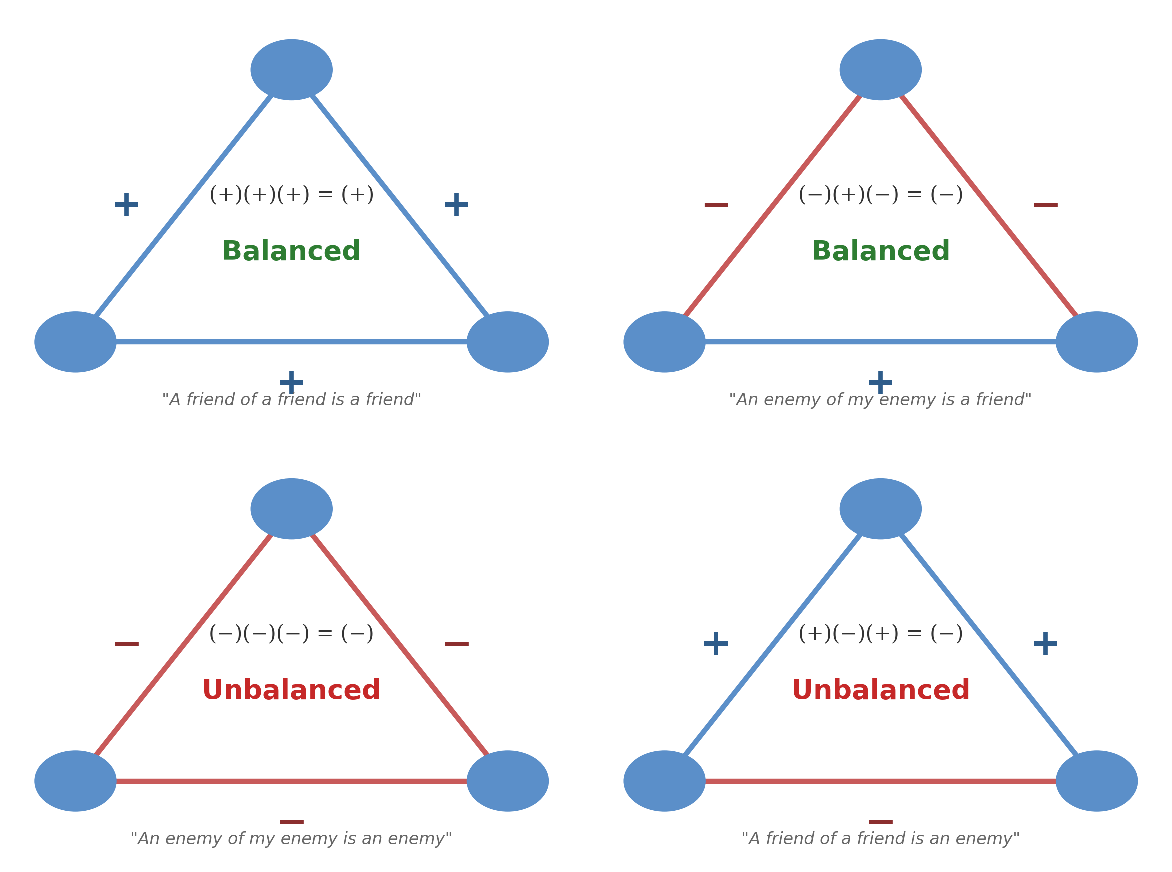After completing this tutorial, you will be able to:- Implement advanced structural terms in ERGM models (GWESP, GWDSP, triadic structures)- Perform and interpret MCMC convergence diagnostics- Compare nested models and assess model fit- Interpret complex ERGM results in substantive terms- Handle model degeneracy using **tapered ERGMs**```{r setup, message=FALSE, warning=FALSE}rm(list =ls())library(network) # Network object manipulationlibrary(ergm) # ERGM fittinglibrary(networkdata) # Network datasetslibrary(sna) # Social network analysis toolslibrary(parallel) # Speed up MCMClibrary(ergm.tapered) # Tapered ERGM for handling degeneracylibrary(amen)# Install ergm.tapered if needed# devtools::install_github("statnet/ergm", ref="tapered")```::: callout-note**Why ergm.tapered?**The `ergm.tapered` package provides an alternative estimation method that better handles models with strong dependence between terms. When you include multiple structural terms (like gwesp and gwdsp), standard ERGM estimation can struggle with convergence. Tapered ERGM adds a "tapering" mechanism that helps stabilize estimation.Software available on GitHub as ergm.tapered: https://github.com/statnet/ergm.taperedYou can use these following code to install `ergm` or `ergm.tapered`:```install.packages("ergm", repos="http://www.stat.ucla.edu/~handcock")install.packages("ergm.tapered", repos="http://www.stat.ucla.edu/~handcock")```or ```install.packages("devtools")devtools::install_github("statnet/ergm.tapered")```:::## 1. Introduction for Advanced Structural Terms in ERGMs### 1.1 Understanding Geometrically Weighted StatisticsBefore diving into applications, let's understand the sophisticated structural terms available in ERGMs. These terms capture complex network dependencies while avoiding the degeneracy issues that plague simpler specifications.::: {.callout-note}**Why Geometrically Weighted Terms?**Traditional count statistics (like triangle counts) can lead to model degeneracy because they treat all configurations equally. Geometrically weighted terms apply **diminishing returns** - the first few shared partners matter more than additional ones, making the model more stable and interpretable.:::### 1.2 Main Function Reference TableHere's a detailed reference table for advanced ERGM structural terms:| Function | Syntax | Description | Interpretation | When to Use ||----------|---------|-------------|----------------|-------------|| **istar(k)** |`istar(2)`| k-in-stars: counts nodes with exactly k incoming edges | Popularity effects in directed networks | Testing for preferential attachment to popular nodes || **ostar(k)** |`ostar(2)`| k-out-stars: counts nodes with exactly k outgoing edges | Activity effects in directed networks | Testing for variation in node activity levels || **gwodegree(decay)** |`gwodegree(0.5, fixed=TRUE)`| Geometrically weighted out-degree distribution | Controls out-degree heterogeneity with diminishing returns | Modeling sender activity patterns without degeneracy || **gwidegree(decay)** |`gwidegree(0.5, fixed=TRUE)`| Geometrically weighted in-degree distribution | Controls in-degree heterogeneity with diminishing returns | Modeling popularity/receiver effects without degeneracy || **gwesp(decay)** |`gwesp(0.5, fixed=TRUE)`| Geometrically weighted edgewise shared partners | Transitivity: "friend of friend is friend" with diminishing returns | Capturing clustering while avoiding degeneracy || **gwdsp(decay)** |`gwdsp(0.5, fixed=TRUE)`| Geometrically weighted dyadwise shared partners | Shared partners between any dyad (connected or not) | Modeling local clustering and "small world" effects || **ctriple** |`ctriple` or `ctriad`| Cyclic triples: A→B→C→A patterns | Non-hierarchical, cyclic relationships | Testing for cyclic vs hierarchical structures || **ttriple** |`ttriple` or `ttriad`| Transitive triples: A→B→C with A→C | Hierarchical, transitive closure | Testing for transitivity and balance theory |::: {.callout-note}Check the model terms using `help("ergm-terms")`:::::: {.callout-tip}Choosing Decay ParametersThe decay parameter (α) in geometrically weighted terms controls how quickly the weight diminishes:- **α = 0**: Only the first shared partner matters- **α = 0.5**: Moderate decay (common choice)- **α = 1.0**: Slower decay, more weight on higher numbers- **α → ∞**: Approaches regular count statisticsStart with α = 0.5 as a default and adjust based on model diagnostics.:::## 2. Tapered ERGM: Solving the Degeneracy Problem### 2.1 Why We Need Tapered ERGMOne of the most frustrating challenges in ERGM modeling is **model degeneracy** (or near-degeneracy). This occurs when a model places almost all its probability mass on extreme network configurations—like empty graphs, complete graphs, or other boundary cases. #### 2.1.1 The Triangle ProblemA classic example is the triangle model:$$P_\eta(Y = y) = \frac{\exp\{\eta_1\text{edge}(y) + \eta_2\text{triangle}(y)\}}{c(\eta_1, \eta_2)}$$This model is near-degenerate for most values of $\eta_2 > 0$. When we try to include theoretically meaningful terms like triangles, GWESP, or other clustering measures, the model often becomes unstable and produces unreliable results.#### 2.1.2 Practical ConstraintsNear-degeneracy has constrained practical ERGM modeling:- **Limited term selection**: Many intuitive or theory-driven terms (like triangles) often cannot be used.- **Model instability**: MCMC algorithms fail to converge or produce degenerate samples.- **Multimodality**: The distribution over network statistics becomes bimodal or multimodal, making inference unreliable.This is why we've had to be so careful about model specification in previous tutorials—we've been working around the degeneracy problem rather than solving it directly.### 2.2 How Tapered ERGM Works#### 2.2.1 The Model SpecificationThe Tapered ERGM has the form:$$q(y|\theta, \tau) = \frac{1}{Z(\theta, \tau)} \exp\left\{\sum_k \theta_k g_k(y) - \sum_k \tau_k(\mu_k(\theta, \tau) - g_k(y))^2\right\}$$where:- $\theta$ = standard ERGM parameters (same interpretation as before)- $\tau$ = tapering parameters (hyperparameters that control stability)- $\mu(\theta, \tau) = E_q[g(Y)]$ = mean value parameters- The second term $-\sum_k \tau_k(\mu_k - g_k(y))^2$ is the **tapering term**The tapering term acts as a **soft constraint** that penalizes network configurations far from the mean $\mu$. Think of it as:- An "attractive force" pulling the distribution toward its mode- The strength of this force is controlled by $\tau_k$- When $\tau = 0$, we recover the standard ERGM- As $\tau$ increases, the model becomes more stable but potentially more biased#### 2.2.2 Maximum Entropy InterpretationThe tapering term has a beautiful theoretical interpretation. The Tapered ERGM arises from a **constrained maximum entropy** problem:$$\begin{align}\text{maximize}_q &\quad -\sum_y q(y)\log(q(y)) \\\text{subject to} &\quad E_q[g_i(Y,X)] = \mu_i \\&\quad E_q[(\mu_i - g_i(Y,X))^2] \leq \sigma^2_i, \quad \forall i\end{align}$$In other words, we're finding the distribution that:1. Has maximum entropy (is least constrained)2. Matches expected network statistics3. **Also constrains the variance** of those statistics to be at most $\sigma^2_i$This variance constraint is what prevents degeneracy.### 2.3 Choosing the Tapering Parameters#### 2.3.1 Parameter Interpretation**When Tapering is Zero ($\tau = 0$)**The model reduces to standard ERGM, and $\theta_k$ represents conditional log-odds as usual.**When Tapering is Non-Zero ($\tau > 0$)**The interpretation changes slightly. The conditional log-odds of a tie becomes:$$\log\left(\frac{P(Y_{ij}=1|Y^c_{ij})}{P(Y_{ij}=0|Y^c_{ij})}\right) = \sum_k \Delta t_k(Y_{ij})[\theta_k + \tau_k \delta_{kij}]$$The term $\tau_k \delta_{kij}$ represents a **bias** introduced by tapering. However, this bias:- Is typically small when the model is well-specified- Ensures computational stability- Is a worthwhile trade-off for being able to use meaningful network terms#### 2.3.2 Choosing the Tapering ParametersHow do we determine $\tau$? The lecture materials suggest using **kurtosis** as a measure of potential degeneracy:$$\text{Kurt}[g(Y)] = \frac{\mu_4}{\mu_2^2} = E[Z^4] \text{ where } Z \text{ is standardized}$$Key facts about kurtosis:- $\text{Kurt}[g(Y)] \geq 1$ always- Gaussian: $\text{Kurt} = 3$- Uniform: $\text{Kurt} = 1.8$- Higher kurtosis suggests bimodality/degeneracyThe tapering is determined by constraining variance:$$V(\theta, \tau) = Var_q(g(Y)) = \sigma^2$$The `ergm.tapered` package automatically estimates appropriate $\tau$ values based on:1. The observed network statistics2. Desired variance constraints3. Ensuring non-degeneracyAutomatic Selection: in practice, the package `ergm.tapered()` will- Usually choose standard ERGM ($\tau = 0$) when justified- Only add tapering when needed for stability- Balance bias-variance trade-off automatically### 2.4 Summary: When to Use Tapered ERGM**Use Tapered ERGM when (recommended):**- You want to include theoretically important but potentially problematic terms (triangles, GWESP, etc.)- Standard ERGM shows convergence issues or degeneracy warnings- You need guaranteed computational stability- You're modeling larger networks where degeneracy is more likely**Advantages:**- Theoretical guarantee of non-degeneracy- Minimal bias when standard ERGM would work- Interpretable as constrained maximum entropy- Available in user-friendly software (`ergm.tapered` package)**Trade-offs:**- Slight bias in parameter estimates (usually small)- Additional hyperparameters ($\tau$) to consider- Need to understand what tapering means for interpretationThe Tapered ERGM represents a major breakthrough in network modeling, finally allowing us to use the full richness of ERGM specifications without worrying too much about the degeneracy. ## 3. Case Study 1 - The French Financial Elite Network### 3.1 The French Financial Elite Network Basic InformationWe'll work with a network collected by Charles Kadushin (1995) of 28 members of the French financial elite. This network captures friendship ties and includes rich vertex attributes that allow us to explore multiple dimensions of homophily.**Data Source:**Kadushin, C. 1995. Friendship among the French financial elite. *American Sociological Review* 60:202-221.```{r, message=FALSE, warning=FALSE}data(ffef)help(ffef)network.size(ffef)network.edgecount(ffef)gden(ffef)list.vertex.attributes(ffef)```The network includes several important vertex covariates:- **prestige**: 0 (neither particule nor social register), 1 (either), or 2 (both)- **party**: Political party membership (11 parties)- **ena**: Graduated from ENA (École nationale d'administration)? 1=yes, 2=no- **masons**: Mason membership- **religion**: Religious affiliation- **topboards**: Number of top corporate boards```{r, message=FALSE, warning=FALSE, fig.width=10, fig.height=8}ena_status <- ffef %v%"ena"vertex_colors <-ifelse(ena_status ==1, "coral", "skyblue")plot(ffef, vertex.col = vertex_colors, main ="French Financial Elite Network Colored by ENA Status", vertex.cex =1.5, edge.col ="gray70")```**Observations:**1. **Visible clustering by ENA attendance**: Individuals who graduated from ENA tend to form connections with other ENA graduates, suggesting strong educational homophily2. **Centrality patterns**: ENA graduates appear more concentrated in the network core, while non-ENA graduates are more dispersed around the periphery3. **Cross-group ties exist**: While there's clear same-status clustering, we also observe connections between ENA and non-ENA graduates### 3.2 Building a Sophisticated ERGM Model```{r french-ergm, message=FALSE, warning=FALSE}#using ergm.tapered() for better handling of strong dependenciesfit_elite <-ergm.tapered( ffef ~ edges +# Baseline densitynodematch("ena") +# ENA homophilynodematch("prestige") +# Prestige homophilynodematch("party") +# Political party homophilygwesp(0.5, fixed =TRUE) +# Transitive closure (clustering)gwdsp(0.5, fixed =TRUE), # Shared partnersverbose =FALSE)summary(fit_elite)```### 3.3 Interpreting Model Coefficients```{r interpretation, message=FALSE}coef_table <-data.frame(Term =names(coef(fit_elite)),Coefficient =round(coef(fit_elite), 3),SE =round(summary(fit_elite)$coefficients[, "Std. Error"], 3),OR =round(exp(coef(fit_elite)), 3),p_value =round(summary(fit_elite)$coefficients[, "Pr(>|z|)"], 4))print(coef_table)baseline_prob <-plogis(coef(fit_elite)["edges"])ena_match_prob <-plogis(coef(fit_elite)["edges"] +coef(fit_elite)["nodematch.ena"])prestige_match_prob <-plogis(coef(fit_elite)["edges"] +coef(fit_elite)["nodematch.prestige"])party_match_prob <-plogis(coef(fit_elite)["edges"] +coef(fit_elite)["nodematch.party"])cat("Baseline (no matches):", round(baseline_prob, 4), "\n")cat("Same ENA status:", round(ena_match_prob, 4), "\n")cat("Same prestige level:", round(prestige_match_prob, 4), "\n")cat("Same party affiliation:", round(party_match_prob, 4), "\n")```- **Edges:** $\beta = -4.63$ represent the baseline log-odds of a friendship tie existing between any two randomly selected individuals in the networks, while controlling other predictors. The strong negative coefficient indicates this is a very sparse network. The $OR = 0.010$ means the baseline odds of a tie is about 1.0%. The baseline robability of friendship is approximately 0.96%.- **nodematch.ena:** $\beta = 1.57$ measures homophily on ENA attendance. The $OR = 4.79$ means that two individuals who share ENA status (both graduate from ENA or both did not) have 4.79 times higher odds of being friends compared to two individuals with different ENA status. The coefficient is strong and highly significant. And the probability of a friendship tie between two individuals who share the same ENA status is 4.45%.- **nodematch.prestige:** $\beta = 0.68$ measures homophily on prestige level (having particule and/or social register listing).The coefficient is moderate and significant (p = 0.015). The $OR = 1.97$ mean that two individuals with the same prestige level have 1.97 times higher odds of being friends compared to those with different prestige levels. The probability of a friendship tie between two individuals who share the same prestige level is 1.88%.- **nodematch.party:** $\beta = 1.25$ measures homophily on political party affiliation. The coefficient is strong and highly significant (p \< 0.001).The $OR = 3.49$ means that two individuals from the same political party have 3.49 times higher odds of being friends compared to those from different parties. The probability of a friendship tie between two individuals who share the same party affiliation is 3.28%.- **GWESP(0.5):** $\beta = 0.43$ measures transitivity and clustering through Geometrically Weighted Edgewise Shared Partners. This term captures the "friend of a friend is a friend" phenomenon. The coefficient is moderate and significant (p = 0.013). The $OR = 1.53$ indicates that networks with more shared partners (triangles) are more probable. The French financial elite network exhibits strong transitivity. If person A is friends with person B, and person B is friends with person C, then A and C are significantly more likely to also be friends.- **GWDSP(0.5):** $\beta = 0.19$ measures local network structure through Geometrically Weighted Dyadwise Shared Partners. This term captures the tendency for dyads (pairs) to share partners, even if they're not directly connected. The coefficient is modest but significant (p = 0.003). The $OR = 1.21$ indicates preference for configurations where individuals share common friends. Beyond direct transitivity, there's a tendency for individuals to be embedded in overlapping social circles. This creates a "small world" structure where even if two people aren't direct friends, they're likely to share mutual acquaintances.::: callout-note``` plogis(coef["edges"] + coef["gwesp.fixed.0.5"])```**This does NOT work because:**- GWESP is not a 0/1 indicator variable- GWESP is a **count statistic** that depends on the entire network structure- GWESP uses a **geometrically weighted** function: $\sum_{k=1}^{n-2} \{1 - (1-e^{-\alpha})^k\} \cdot EP_k$Summary:| Term Type | Example Terms | Can use `plogis(edges + term)`? | Why/Why not? ||------------------|------------------|------------------|------------------|| **Node attributes** |`nodematch()`, `nodecov()`, `absdiff()`| YES | Binary 0/1 or known numeric covariate values || **Dyad attributes** |`edgecov()`, `dyadcov()`| YES (with care) | Known covariate value for specific dyad || **Structural terms** |`gwesp()`, `gwdsp()`, `triangle`, `ttriad`, `ctriad`| NO | Value depends on entire network configuration || **Degree terms** |`gwdegree()`, `degree()`, `idegree()`, `odegree()`| NO | Depends on node's position in network |:::### 3.4 MCMC Diagnostics - Ensuring Model Reliability```{r mcmc-diagnostics, fig.width=12, fig.height=10, message=FALSE, warning=FALSE}mcmc_diag <-mcmc.diagnostics(fit_elite, vars.per.page =6)```::: {.callout-note}MCMC Diagnostic Components Explained:- **Sample Statistics vs. Observed**: Compares simulated network statistics to observed values. Good fit shows statistics centered around zero.- **Trace Plots**: Show MCMC chain values over iterations. Good mixing looks like "fuzzy caterpillar" around zero.- **Density Plots**: Distribution of sampled statistics. Should be approximately normal and centered near zero.- **Autocorrelation Function (ACF)**: Measures correlation between successive samples. Should decay quickly to near zero.- **Geweke Diagnostic**: Tests whether early and late parts of chain come from same distribution (burn-in test).:::Let's extract some key diagnostic statistics:```{r diagnostic-summary}gof_elite <-gof(fit_elite, GOF =~degree + esp + dsp + triadcensus, verbose =FALSE)plot(gof_elite)```From the sample statistics vs. observed values, the statistics show good agreement between simulated and observed values. All terms have p-value \> 0.05, The overall chi-squared test p = 0.022, indicating the model successfully reproduces the observed network statistics. The trace plots show relatively good mixing, fluctuating randomly around zero, which means MCMC chains are exploring the parameter space well and not getting trapped in any particular region. All the density plots are approximately centered near zeor, and no extreme skewness and multinodality (multiple peaks), indicating the sampling stable parameter estimation. Moreover, for the Geweke Diagnostic (Burn-in Test), all p-values are well above 0.05, indicating no evidence of non-convergence. The joint p-value of 0.820 indicates good overall convergence. Overall, the model successfully converged and the parameter estimates are reliable for inference.## 4. Social Balance and Transitivity in Network Analysis### 4.1 Definition of Social BalanceSocial balance and transitivity are concepts in network analysis that help us understand how relationships form and evolve in social networks. These concepts, rooted in social psychology and graph theory, provide insights into the micro-level mechanisms that shape macro-level network structures.#### Heider's Balance TheoryFritz Heider's balance theory examines relationships among three actors (P-O-X triads) where each dyadic relationship can be positive (+) or negative (-). According to Heider:- **Balanced triads** have stable configurations: - All three relationships are positive: (+)(+)(+) = (+) — "A friend of a friend is a friend" - Two negative relationships: (-)(+)(-) = (-) — "An enemy of my enemy is a friend"- **Unbalanced triads** create psychological tension: - All negative: (-)(-)(-)= (-) — "An enemy of my enemy is an enemy" - One negative: (+)(-)(+) = (-) — "A friend of a friend is an enemy"The key principle: **multiply the signs of all three edges**. If the product is positive, the triad is balanced; if negative, it's unbalanced.*The following plot shows the four foundamental triad configurations in balance theory. Balanced triads (top row) are psychologically stable, while unbalanced triads (bottom row) create cognitive tension that motivates relationship change.*### 4.2 From Undirected to Directed NetworksWhile Heider's original theory focused on undirected relationships, real social networks often involve directed ties (e.g., "A nominates B as a friend" doesn't guarantee reciprocity). For directed networks, we use:- **MAN notation**: Classifies triads by the number of Mutual, Asymmetric, and Null dyads- **16 triad types**: From 003 (no connections) to 300 (completely connected), the following plots represent the 16 types- **Notation** The first number represents the number of mutual (bidirectional) edges within the triad. These are pairs of vertices with a connection in both directions (e.g., A is connected to B, and B is connected to A). The second number in the three-digit code indicates the number of asymmetric (unidirectional) edges, and the third number represents the number of null (non-existent) edges. 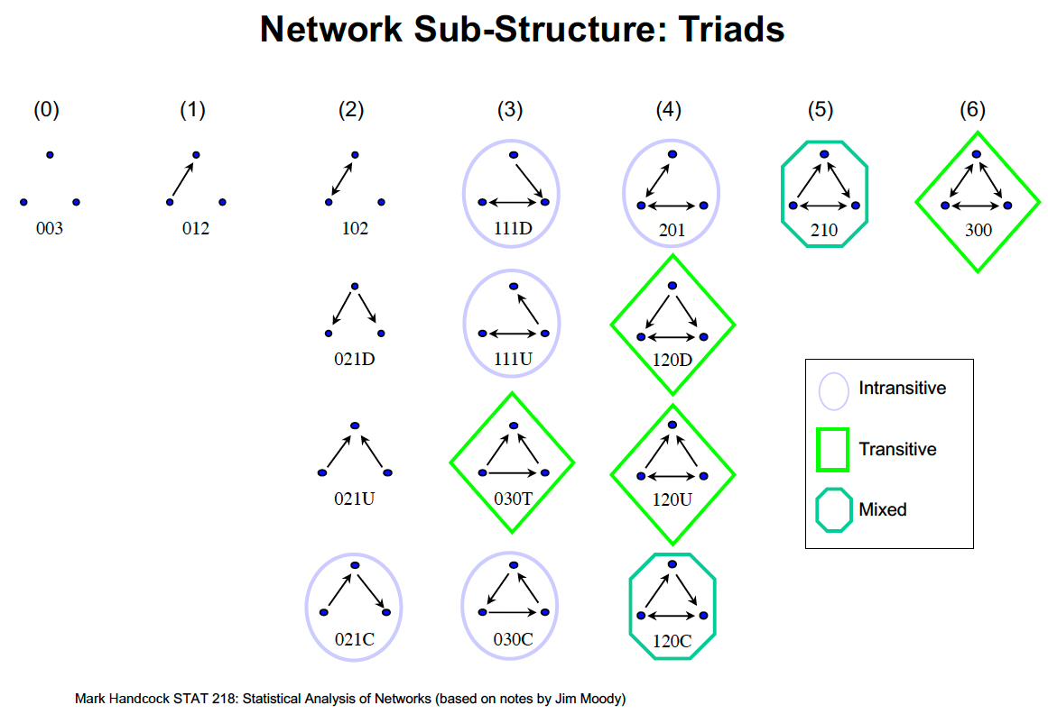#### Transitivity in Directed NetworksTransitivity captures the "friend of a friend" phenomenon:- If i → j and j → k, then i → k (transitive closure)- **Transitive triads**: e.g., 030T, 120D, 120U, 300, indicate hierarchical or clustered structures- **Intransitive triads** e.g., 111D, 111U, 030C, suggest competing relationships or ranked preferences- **Cyclic triads** e.g.m 030C: A→B→C→A, represent circular patterns without hierarchical closure### 4.3 Network-Level ImplicationsBalance theory has profound implications for understanding macro-level network structure:1. **Clustered Communities**: If balance holds throughout a network, we expect clear group boundaries with positive ties within groups and negative ties between groups2. **Structural Balance Theorem**: A completely balanced signed network must have one of two structures: - A single cohesive clique (all positive ties) - Two opposing factions (positive within, negative between)3. **Weak Balance**: Real networks often show "weak balance" where the all-negative triad (-)(-)(-) is also allowed, permitting multiple clusters rather than just two factions### 4.4 Measuring Balance in Real NetworksWe can empirically test balance theory using:- **Triad census**: Count the frequency of each triad type- **Statistical comparison**: Compare observed counts to expected distributions under random graphs- **ERGM terms**: - `ttriad` (transitive triads count) - `ctriad` (cyclic triads count)## 5. Case Study 2 - Balance Theory in Hansell Classroom FriendshipsNow let's examine balance theory using directed friendship nominations in a sixth-grade classroom, we've used this dataset in the [previous tutorial (Part 5)](https://aliceaii.github.io/posts/snapart5/):### 5.1 Is the friendship network balanced in Heider’s definition of balance?::: {.callout-tip}**Heider's Balance Theory**In a balanced network:- **Transitive triads** (A→B→C implies A→C): "Friend of friend is friend"- **Avoided cyclic triads** (A→B→C→A without A→C): Creates tensionBalanced networks have positive transitive triad coefficients and negative cyclic triad coefficients.:::```{r, message=FALSE, warning=FALSE}library(networkdata)data(hansell)help(hansell)#summary(hansell)table(hansell %v%"sex")triad.census(hansell)#transitive triadstriads <-triad.census(hansell)triads[9] # 030T#cyclic triadstriads[10] # 030C ```### 5.2 Fit the model```{r balance-ergm, message=FALSE, warning=FALSE, cache=TRUE}fit_balance <-ergm.tapered( hansell ~ edges +# Baseline density mutual +# Reciprocitynodematch("sex", diff =TRUE) +# Sex homophily (differentiated) ttriple +# Transitive triples ctriple, # Cyclic triplesverbose =FALSE)summary(fit_balance)balance_coef <-data.frame(Term =c("Edges", "Mutual", "Same Sex (Female)", "Same Sex (Male)", "Transitive Triples", "Cyclic Triples"),Coefficient =round(coef(fit_balance), 3),OR =round(exp(coef(fit_balance)), 3))print(balance_coef, row.names =FALSE)```::: {.callout-important}Evidence for Balance modelThe model provides strong evidence for balance theory:- **Positive transitivity** (β = 0.33, p < 0.05): Transitive closure is preferred- **Negative cyclicity** (β = -0.40, p < 0.001): Cyclic patterns are avoided- **Strong sex homophily**: Both boys and girls prefer same-sex friendships- **No reciprocity effect**: Friendships aren't necessarily mutual at this ageThis pattern suggests the classroom network organizes into balanced, sex-segregated friendship groups with clear hierarchical structures rather than cyclic patterns.:::- **Transitive ties (ttriple):** $\beta = 0.33$, the coefficient measures the tendency for transitive triadic closure in the network, it's significant. The $OR = 1.39$ means that for each additional transitive triple configuration, the odds of the network configuration increased by 39%. When student A nominates student B as a friend, and B nominates C, there is a significantly higher-than-random probability that A will also nominate C. This creates cohesive friendship groups with closed triadic structures.- **Cyclic ties (ctriple):** $\beta = -0.40$, the coefficient measures the tendency for cyclic triadic structures in the network, where: $A→B→C→A$ forms a cycle, but without the full transitive closure. The negative and highly significant coefficient (p \< 0.001) indicates a strong avoidance of cyclic triadic structures. $OR = 0.67$ means that cyclic triple configurations decrease the odds of the network configuration by 33%. The negative coefficient shows that cyclic patterns are less common than would be expected in a random network.### 5.3 Model Comparison and Selection```{r model-comparison, message=FALSE, warning=FALSE}# Fit alternative model for French elite networkfit_elite_extended <-ergm.tapered( ffef ~ edges +nodematch("ena") +nodematch("prestige") +nodematch("party") +nodematch("masons") +# Add Masonic membershipnodematch("religion") +# Add religionnodecov("topboards") +# Board memberships as covariateabsdiff("topboards") +# Difference in board membershipsgwesp(0.5, fixed =TRUE) +gwdsp(0.5, fixed =TRUE),verbose =FALSE)# Model comparisonanova_result <-anova(fit_elite, fit_elite_extended)print(anova_result)# AIC comparisonaic_comparison <-data.frame(Model =c("Base", "Extended"),AIC =c(AIC(fit_elite), AIC(fit_elite_extended)),BIC =c(BIC(fit_elite), BIC(fit_elite_extended)),Parameters =c(length(coef(fit_elite)), length(coef(fit_elite_extended))))print(aic_comparison)```::: {.callout-note}Model Selection Guidelines- **Lower AIC/BIC** indicates better model fit accounting for complexity- **ANOVA p-value > 0.05** suggests additional terms don't significantly improve fit- **Check MCMC diagnostics** for both models - better convergence often trumps marginal fit improvements- **Substantive interpretation** matters - include terms that make theoretical senseIn our case, the simpler model is preferred: lower AIC, similar fit, better convergence.:::## 6. Case Study 3 - Protein-Protein Interaction NetworksButland et al (2005) “Interaction network containing conserved and essential protein complexes in Escherichia coli”reported a network of protein-protein interactions (bindings) that we obtained from http://pil.phys.uniroma1.it/~gcalda/cosinsite/extra/data/proteins/.This data is available in the networkdata package.Convert the edgelist to a directed network (The `el2sm` function may be helpful).Fit various tapered ERGM models to the network using ergm.tapered. Consider terms documented under ergm-terms. Good candidates include `istar`, `ostar`, `gwodegree`, `gwidegree`, `dgwest`, `dgwdsp`, `ctriple`, `ttriple`. Check the MCMC diagnostics with mcmc.diagnostics. Overall, how does the goodness-of-fit look?- Model 1 is a basic model, only include `edges` + `mutual` terms, The `mutual` term has an estimate of -Inf, may indicate the network don't have many mutual ties.- Model 2 is a degree distribution model, includes `edges` + `gwidegree` + `gwodegree`, MCMC diagnostics show relatively good convergence, sample statistics not significantly different from observed (overall p = 0.548) and the trace plot show good mixing.- Model 3 added `dgwesp` + `dgwdsp` + `ctriple` + `ttriple` based on the model 2, the `ctriple` term has estimate -14.20 with NA standard error, which may suggest there are zero or nearly zero cyclic triads in the network. MCMC diagnostics show reasonable convergence, with overall chi-squared test p = 0.530. Lower AIC (6770 vs 7083) suggests better fit than Model 2.```{r, message=FALSE, warning=FALSE}library(networkdata)library(amen)library(network)data(butland_ppi)help(butland_ppi)head(butland_ppi)#get all unique vertices and create mappingall_vertices <-sort(unique(c(butland_ppi[, 1], butland_ppi[, 2])))n_vertices <-length(all_vertices)vertex_map <-data.frame(original_id = all_vertices, new_id =1:n_vertices)#remap edgelist to sequential IDsedgelist_remapped <- butland_ppiedgelist_remapped[, 1] <-match(butland_ppi[, 1], vertex_map$original_id)edgelist_remapped[, 2] <-match(butland_ppi[, 2], vertex_map$original_id)#convert edgelist to sociomatrixsm <-el2sm(edgelist_remapped)#create network objectppi_net <-network(sm, directed =TRUE)network.size(ppi_net)network.edgecount(ppi_net)network.edgecount(ppi_net)``````{r, message=FALSE, warning=FALSE}library(parallel)library(ergm.tapered)set.seed(123)#model 1: basic model with edges and reciprocity#fit_ppi1 <- ergm.tapered(ppi_net ~ edges + mutual, r= 1)fit_ppi1 <-ergm(ppi_net ~ edges + mutual)summary(fit_ppi1)#mcmc.diagnostics(fit_ppi1)#model 2: add in-degree / outdegree distribution effectsfit_ppi2 <-ergm.tapered(ppi_net ~ edges +gwidegree(0.5, fixed =TRUE) +gwodegree(0.5, fixed =TRUE))summary(fit_ppi2)#mcmc.diagnostics(fit_ppi2)#model 3: add GW edgewise shared partners + GW Dyadwise Shared Partnersfit_ppi3 <-ergm.tapered(ppi_net ~ edges +gwidegree(0.5, fixed =TRUE) +gwodegree(0.5, fixed =TRUE) +dgwesp(0.5, fixed =TRUE) +dgwdsp(0.5, fixed =TRUE) + ctriple + ttriple)summary(fit_ppi3)mcmc.diagnostics(fit_ppi3)```## References- Hansell, S. (1984). Cooperative groups, weak ties, and the integration of peer friendships. *Social Psychology Quarterly*, 47(4), 316-328.- Kadushin, C. (1995). Friendship among the French financial elite. *American Sociological Review*, 60, 202-221.- Snijders, T.A.B., Pattison, P.E., Robins, G.L., & Handcock, M.S. (2006). New specifications for exponential random graph models. *Sociological Methodology*, 36(1), 99-153.- Hunter, D.R., & Handcock, M.S. (2006). Inference in curved exponential family models for networks. *Journal of Computational and Graphical Statistics*, 15(3), 565-583.- Blackburn, B., & Handcock, M. S. (2023). Practical network modeling via tapered exponential-family random graph models. *Journal of Computational and Graphical Statistics*, 32(2), 388-401.---*This tutorial is based on UCLA [STATS 218: Social Network Analysis](https://handcock.github.io/teaching/218/) taught by Prof [Mark Handcock](https://handcock.github.io/).*


4. Social Balance and Transitivity in Network Analysis
4.1 Definition of Social Balance
Social balance and transitivity are concepts in network analysis that help us understand how relationships form and evolve in social networks. These concepts, rooted in social psychology and graph theory, provide insights into the micro-level mechanisms that shape macro-level network structures.
Heider’s Balance Theory
Fritz Heider’s balance theory examines relationships among three actors (P-O-X triads) where each dyadic relationship can be positive (+) or negative (-). According to Heider:
The key principle: multiply the signs of all three edges. If the product is positive, the triad is balanced; if negative, it’s unbalanced.
The following plot shows the four foundamental triad configurations in balance theory. Balanced triads (top row) are psychologically stable, while unbalanced triads (bottom row) create cognitive tension that motivates relationship change.
4.2 From Undirected to Directed Networks
While Heider’s original theory focused on undirected relationships, real social networks often involve directed ties (e.g., “A nominates B as a friend” doesn’t guarantee reciprocity). For directed networks, we use:
Transitivity in Directed Networks
Transitivity captures the “friend of a friend” phenomenon:
4.3 Network-Level Implications
Balance theory has profound implications for understanding macro-level network structure:
Clustered Communities: If balance holds throughout a network, we expect clear group boundaries with positive ties within groups and negative ties between groups
Structural Balance Theorem: A completely balanced signed network must have one of two structures:
Weak Balance: Real networks often show “weak balance” where the all-negative triad (-)(-)(-) is also allowed, permitting multiple clusters rather than just two factions
4.4 Measuring Balance in Real Networks
We can empirically test balance theory using:
ttriad(transitive triads count)ctriad(cyclic triads count)