HSLS:09 Study Replication Example 1 (Pinneo & Nolen, 2024)

ED230A
Author

Shuhan (Alice) Ai

Published

November 18, 2025

1. Study Introduction

Pinneo, L., & Nolen, A. (2024). Parent involvement and student academic motivation towards science in 9th grade. Humanities and Social Sciences Communications, 11(1), 1-12. https://doi.org/10.1057/s41599-024-02707-0

Abstract: Parents’ beliefs and behavior act as both explicit and implicit ways of communicating the value of science and their confidence that their child can be successful in science-related classes. Using the NCES High School Longitudinal Survey (HSLS:09), we examined how parent beliefs and behaviors regarding their 9th grader’s science education predicted the students’ motivation in science. Using multiple regression indicates that the combination of parental education, beliefs, and involvement in science-related activities with their child are weak but significant predictors of students’ academic motivation in science (adjR2 = 0.04, F(6, 14,933) = 26.32, P < 0.001). In particular, parent education and parent involvement have positive and significant effects on students’ science identity and science self-efficacy. These findings suggest that students may have a stronger academic motivation in science with parents who have higher levels of education, more confidence in their ability to help their child in science, and who engage in more science activities with their child.

Research questions:

  • RQ1: How do parents’ participation in their 9th grade child’s academic science activities (both at home and at school) affect their child’s academic motivation towards science?

  • RQ2: How do parents’ beliefs about their own confidence in helping their 9th grade child with their science homework affect their child’s academic motivation towards science?

Sample and Method: Using HSLS:09 base year, the data included 14,028 9th grade students.

The analysis for this project was conducted in two parts.

  • The first part includes the descriptive analysis for parent characteristics, beliefs, and behaviors. These variables were crosstabulated to further examine how parent beliefs and behaviors varied by parent education.

  • The second part of the analysis included a multiple linear regression to examine the combinations of factors that predict student science motivation. The description of the analysis also includes checking all assumptions for multiple regression analysis (i.e., multicollinearity, outliers, and homogeneity of variance).

Variable Lists:

Independent Variables (Predictors):

  • X1PAREDU: Parent education - highest level of education achieved by either parent
  • P1E04B/P1SCIHWEFF: Parent science efficacy - confidence in helping with 9th grade science homework
  • P1E05B/P1SCICOMP: Parent beliefs about gender - comparison of females’ and males’ abilities in science

Parent behaviors composite (6 items, dummy-coded and summed, 0-6):

  • P1E07A/P1MUSEUM: Visited science/engineering museum
  • P1E07B/P1COMPUTER: Worked/played on computer with student
  • P1E07C/P1FIXED: Built or fixed something with student
  • P1E07D/P1SCIFAIR: Attended school science fair
  • P1E07E/P1SCIPROJ: Helped with school science fair project
  • P1E07F/P1STEMDISC: Discussed STEM program or article

Dependent Variables (Outcomes):

  • X1SCIID: Student science identity
  • X1SCIUTI: Student science utility value
  • X1SCIEFF: Student science self-efficacy
  • X1SCIINT: Student science interest”

2. Set up packages and data

rm(list=ls())

library(tidyverse)
library(haven) 
library(psych)
library(car) #for VIF
library(lmtest)
library(table1)
library(stargazer) #for table presentation
library(lm.beta) #for standardized coefficients
library(ppcor)#for correlation calculation

load("/Users/aishuhan/Desktop/UCLA PhD/Dataset/HSLS 2009-2013 Public Use Data ICPSR_36423/DS0002 Student Level Data/36423-0002-Data.rda")

dt <- da36423.0002
remove(da36423.0002)

dt <- dt %>%
  dplyr::select(STU_ID, X1PAREDU, P1SCIHWEFF, P1SCICOMP, 
         P1MUSEUM, P1COMPUTER, P1FIXED, P1SCIFAIR, P1SCIPROJ, P1STEMDISC,
         X1SCIID, X1SCIUTI, X1SCIEFF, X1SCIINT)

#calculate proportion of missing data for each variables
colMeans(is.na(dt))
    STU_ID   X1PAREDU P1SCIHWEFF  P1SCICOMP   P1MUSEUM P1COMPUTER    P1FIXED 
 0.0000000  0.2859635  0.3350211  0.3728460  0.3427222  0.3427222  0.3427222 
 P1SCIFAIR  P1SCIPROJ P1STEMDISC    X1SCIID   X1SCIUTI   X1SCIEFF   X1SCIINT 
 0.3427222  0.3427222  0.3427222  0.1018593  0.2637961  0.2654555  0.2797090 

3. Descriptive Analysis

Table 1 (a) Parent background, beliefs, and behaviors (HSLS:09 base-year)

#we used the data will NA here, the total count for the X1PAREDU should have missing
table1(~ factor(X1PAREDU) + factor(P1SCIHWEFF) + factor(P1SCICOMP), data=dt)
Overall
(N=23503)
factor(X1PAREDU)
(1) Less than high school 1010 (4.3%)
(2) High school diploma or GED 5909 (25.1%)
(3) Associate's degree 2549 (10.8%)
(4) Bachelor's degree 4102 (17.5%)
(5) Master's degree 2116 (9.0%)
(7) Ph.D/M.D/Law/other high lvl prof degree 1096 (4.7%)
Missing 6721 (28.6%)
factor(P1SCIHWEFF)
(1) Very confident 6166 (26.2%)
(2) Somewhat confident 7321 (31.1%)
(3) Not at all confident 2142 (9.1%)
Missing 7874 (33.5%)
factor(P1SCICOMP)
(1) Females are much better 376 (1.6%)
(2) Females are somewhat better 582 (2.5%)
(3) Females and males are the same 10612 (45.2%)
(4) Males are somewhat better 2587 (11.0%)
(5) Males are much better 583 (2.5%)
Missing 8763 (37.3%)
behavior_vars <- c("P1MUSEUM", "P1COMPUTER", "P1FIXED", "P1SCIFAIR", "P1SCIPROJ", "P1STEMDISC")

for(v in behavior_vars) {
  print(v)
  print(table(dt[[v]]))
  print(prop.table(table(dt[[v]])) * 100)
}
[1] "P1MUSEUM"

 (0) No (1) Yes 
   7195    8253 

  (0) No  (1) Yes 
46.57561 53.42439 
[1] "P1COMPUTER"

 (0) No (1) Yes 
   2148   13300 

  (0) No  (1) Yes 
13.90471 86.09529 
[1] "P1FIXED"

 (0) No (1) Yes 
   8461    6987 

  (0) No  (1) Yes 
54.77084 45.22916 
[1] "P1SCIFAIR"

 (0) No (1) Yes 
  12732    2716 

  (0) No  (1) Yes 
82.41844 17.58156 
[1] "P1SCIPROJ"

 (0) No (1) Yes 
   9377    6071 

  (0) No  (1) Yes 
60.70041 39.29959 
[1] "P1STEMDISC"

 (0) No (1) Yes 
   5249   10199 

  (0) No  (1) Yes 
33.97851 66.02149 

Table 1 (b) Student academic motivation in science scaled scores (HSLS:09 Base year)

table1(~ X1SCIID + X1SCIUTI + X1SCIEFF + X1SCIINT, data=dt)
Overall
(N=23503)
X1SCIID
Mean (SD) 0.0424 (1.01)
Median [Min, Max] -0.330 [-1.57, 2.15]
Missing 2394 (10.2%)
X1SCIUTI
Mean (SD) 0.0136 (0.990)
Median [Min, Max] 0.100 [-3.10, 1.69]
Missing 6200 (26.4%)
X1SCIEFF
Mean (SD) 0.0372 (0.998)
Median [Min, Max] 0.250 [-2.91, 1.83]
Missing 6239 (26.5%)
X1SCIINT
Mean (SD) 0.0323 (0.995)
Median [Min, Max] 0.160 [-2.59, 2.03]
Missing 6574 (28.0%)

Table 1 (c) Parents’/guardians’ highest level of education and Their Confidence in helping with 9th grade science homework Crosstabulation

  • removed all the NA for P1SCIHWEFF and X1PAREDU, then proformed the cross tabulation
  • can use table1
dt_psscihw <- dt %>% filter(!is.na(P1SCIHWEFF) & !is.na(X1PAREDU))
table1(~ factor(X1PAREDU) | factor(P1SCIHWEFF), data = dt_psscihw)
(1) Very confident
(N=6165)
(2) Somewhat confident
(N=7320)
(3) Not at all confident
(N=2141)
Overall
(N=15626)
factor(X1PAREDU)
(1) Less than high school 175 (2.8%) 362 (4.9%) 353 (16.5%) 890 (5.7%)
(2) High school diploma or GED 1520 (24.7%) 2895 (39.5%) 968 (45.2%) 5383 (34.4%)
(3) Associate's degree 939 (15.2%) 1179 (16.1%) 247 (11.5%) 2365 (15.1%)
(4) Bachelor's degree 1802 (29.2%) 1766 (24.1%) 328 (15.3%) 3896 (24.9%)
(5) Master's degree 1091 (17.7%) 783 (10.7%) 167 (7.8%) 2041 (13.1%)
(7) Ph.D/M.D/Law/other high lvl prof degree 638 (10.3%) 335 (4.6%) 78 (3.6%) 1051 (6.7%)

Table 1 (d) Parents’/guardians’ highest level of education and Parents’ beliefs about females’ and males’ abilities in science X Parent education

dt_pscic <- dt %>% filter(!is.na(P1SCICOMP) & !is.na(X1PAREDU))
table1(~ factor(X1PAREDU) | factor(P1SCICOMP), data = dt_pscic)
(1) Females are much better
(N=376)
(2) Females are somewhat better
(N=582)
(3) Females and males are the same
(N=10610)
(4) Males are somewhat better
(N=2587)
(5) Males are much better
(N=583)
Overall
(N=14738)
factor(X1PAREDU)
(1) Less than high school 56 (14.9%) 63 (10.8%) 594 (5.6%) 91 (3.5%) 41 (7.0%) 845 (5.7%)
(2) High school diploma or GED 126 (33.5%) 233 (40.0%) 3555 (33.5%) 869 (33.6%) 243 (41.7%) 5026 (34.1%)
(3) Associate's degree 52 (13.8%) 79 (13.6%) 1560 (14.7%) 424 (16.4%) 107 (18.4%) 2222 (15.1%)
(4) Bachelor's degree 87 (23.1%) 123 (21.1%) 2688 (25.3%) 672 (26.0%) 112 (19.2%) 3682 (25.0%)
(5) Master's degree 36 (9.6%) 56 (9.6%) 1451 (13.7%) 373 (14.4%) 52 (8.9%) 1968 (13.4%)
(7) Ph.D/M.D/Law/other high lvl prof degree 19 (5.1%) 28 (4.8%) 762 (7.2%) 158 (6.1%) 28 (4.8%) 995 (6.8%)

3. Multiple regression

Create the MOTIV_index

#this paper do not mention how they create the MOTIV_index
#the most likely approach is use simple mean (then standardized)

dt <- dt %>% dplyr::mutate(MOTIV_index_raw = rowMeans(dplyr::select(., X1SCIID, X1SCIUTI, X1SCIEFF, X1SCIINT), na.rm = FALSE),
                    MOTIV_index = scale(MOTIV_index_raw)[,1])
dt %>%
  summarise(
    Mean = mean(MOTIV_index, na.rm = TRUE),
    SD = sd(MOTIV_index, na.rm = TRUE),
    Min = min(MOTIV_index, na.rm = TRUE),
    Max = max(MOTIV_index, na.rm = TRUE),
    N = sum(!is.na(MOTIV_index))
  )
          Mean SD       Min     Max     N
1 1.424309e-16  1 -3.339767 2.42961 16290

Table 2 Model Summary and Table 4 Model Coefficients

dt_reg <- dt %>%
  dplyr::select(MOTIV_index, X1PAREDU, P1SCIHWEFF, P1SCICOMP, 
                P1MUSEUM, P1COMPUTER, P1FIXED, P1SCIFAIR, P1SCIPROJ, P1STEMDISC) %>%
  mutate(across(everything(), as.numeric)) %>%
  na.omit()

#model 1: parent education only
model1 <- lm(MOTIV_index ~ X1PAREDU, data = dt_reg)
#model 2: add parent beliefs
model2 <- lm(MOTIV_index ~ X1PAREDU + P1SCIHWEFF + P1SCICOMP, data = dt_reg)
#model 3: full model with parent behaviors
model3 <- lm(MOTIV_index ~ X1PAREDU + P1SCIHWEFF + P1SCICOMP + 
               P1MUSEUM + P1COMPUTER + P1FIXED + P1SCIFAIR + P1SCIPROJ + P1STEMDISC,
             data = dt_reg)

summary(model1)

Call:
lm(formula = MOTIV_index ~ X1PAREDU, data = dt_reg)

Residuals:
    Min      1Q  Median      3Q     Max 
-3.5580 -0.6275  0.0033  0.6384  2.6336 

Coefficients:
            Estimate Std. Error t value Pr(>|t|)    
(Intercept) -0.41510    0.03118  -13.31   <2e-16 ***
X1PAREDU     0.10556    0.00681   15.50   <2e-16 ***
---
Signif. codes:  0 '***' 0.001 '**' 0.01 '*' 0.05 '.' 0.1 ' ' 1

Residual standard error: 0.9834 on 11150 degrees of freedom
Multiple R-squared:  0.02109,   Adjusted R-squared:  0.02101 
F-statistic: 240.3 on 1 and 11150 DF,  p-value: < 2.2e-16
summary(model2)

Call:
lm(formula = MOTIV_index ~ X1PAREDU + P1SCIHWEFF + P1SCICOMP, 
    data = dt_reg)

Residuals:
    Min      1Q  Median      3Q     Max 
-3.6175 -0.6252 -0.0024  0.6438  2.7033 

Coefficients:
             Estimate Std. Error t value Pr(>|t|)    
(Intercept) -0.076772   0.062144  -1.235    0.217    
X1PAREDU     0.093257   0.007015  13.293  < 2e-16 ***
P1SCIHWEFF  -0.101245   0.014154  -7.153 9.01e-13 ***
P1SCICOMP   -0.034600   0.014072  -2.459    0.014 *  
---
Signif. codes:  0 '***' 0.001 '**' 0.01 '*' 0.05 '.' 0.1 ' ' 1

Residual standard error: 0.9809 on 11148 degrees of freedom
Multiple R-squared:  0.0262,    Adjusted R-squared:  0.02594 
F-statistic: 99.98 on 3 and 11148 DF,  p-value: < 2.2e-16
summary(model3)

Call:
lm(formula = MOTIV_index ~ X1PAREDU + P1SCIHWEFF + P1SCICOMP + 
    P1MUSEUM + P1COMPUTER + P1FIXED + P1SCIFAIR + P1SCIPROJ + 
    P1STEMDISC, data = dt_reg)

Residuals:
    Min      1Q  Median      3Q     Max 
-3.6061 -0.6188  0.0022  0.6421  2.6614 

Coefficients:
             Estimate Std. Error t value Pr(>|t|)    
(Intercept) -0.588528   0.091158  -6.456 1.12e-10 ***
X1PAREDU     0.080532   0.007143  11.274  < 2e-16 ***
P1SCIHWEFF  -0.076832   0.014267  -5.385 7.38e-08 ***
P1SCICOMP   -0.030432   0.013984  -2.176 0.029556 *  
P1MUSEUM     0.082181   0.019455   4.224 2.42e-05 ***
P1COMPUTER  -0.077725   0.028437  -2.733 0.006282 ** 
P1FIXED      0.057349   0.019096   3.003 0.002678 ** 
P1SCIFAIR    0.090202   0.026059   3.462 0.000539 ***
P1SCIPROJ    0.034646   0.020569   1.684 0.092135 .  
P1STEMDISC   0.174321   0.021003   8.300  < 2e-16 ***
---
Signif. codes:  0 '***' 0.001 '**' 0.01 '*' 0.05 '.' 0.1 ' ' 1

Residual standard error: 0.9741 on 11142 degrees of freedom
Multiple R-squared:  0.0401,    Adjusted R-squared:  0.03932 
F-statistic: 51.72 on 9 and 11142 DF,  p-value: < 2.2e-16
vif(model2)
  X1PAREDU P1SCIHWEFF  P1SCICOMP 
  1.066522   1.067281   1.001229 
vif(model3)
  X1PAREDU P1SCIHWEFF  P1SCICOMP   P1MUSEUM P1COMPUTER    P1FIXED  P1SCIFAIR 
  1.121097   1.099521   1.002419   1.100050   1.076309   1.061010   1.187355 
 P1SCIPROJ P1STEMDISC 
  1.187516   1.140765 
stargazer(model1, model2, model3, type = "text", digits = 3)

==================================================================================================
                                                 Dependent variable:                              
                    ------------------------------------------------------------------------------
                                                     MOTIV_index                                  
                               (1)                        (2)                       (3)           
--------------------------------------------------------------------------------------------------
X1PAREDU                     0.106***                  0.093***                  0.081***         
                             (0.007)                    (0.007)                   (0.007)         
                                                                                                  
P1SCIHWEFF                                             -0.101***                 -0.077***        
                                                        (0.014)                   (0.014)         
                                                                                                  
P1SCICOMP                                              -0.035**                  -0.030**         
                                                        (0.014)                   (0.014)         
                                                                                                  
P1MUSEUM                                                                         0.082***         
                                                                                  (0.019)         
                                                                                                  
P1COMPUTER                                                                       -0.078***        
                                                                                  (0.028)         
                                                                                                  
P1FIXED                                                                          0.057***         
                                                                                  (0.019)         
                                                                                                  
P1SCIFAIR                                                                        0.090***         
                                                                                  (0.026)         
                                                                                                  
P1SCIPROJ                                                                         0.035*          
                                                                                  (0.021)         
                                                                                                  
P1STEMDISC                                                                       0.174***         
                                                                                  (0.021)         
                                                                                                  
Constant                    -0.415***                   -0.077                   -0.589***        
                             (0.031)                    (0.062)                   (0.091)         
                                                                                                  
--------------------------------------------------------------------------------------------------
Observations                  11,152                    11,152                    11,152          
R2                            0.021                      0.026                     0.040          
Adjusted R2                   0.021                      0.026                     0.039          
Residual Std. Error     0.983 (df = 11150)        0.981 (df = 11148)        0.974 (df = 11142)    
F Statistic         240.275*** (df = 1; 11150) 99.977*** (df = 3; 11148) 51.717*** (df = 9; 11142)
==================================================================================================
Note:                                                                  *p<0.1; **p<0.05; ***p<0.01
#get the standared coefficient
summary(lm.beta(model1))

Call:
lm(formula = MOTIV_index ~ X1PAREDU, data = dt_reg)

Residuals:
    Min      1Q  Median      3Q     Max 
-3.5580 -0.6275  0.0033  0.6384  2.6336 

Coefficients:
            Estimate Standardized Std. Error t value Pr(>|t|)    
(Intercept) -0.41510           NA    0.03118  -13.31   <2e-16 ***
X1PAREDU     0.10556      0.14524    0.00681   15.50   <2e-16 ***
---
Signif. codes:  0 '***' 0.001 '**' 0.01 '*' 0.05 '.' 0.1 ' ' 1

Residual standard error: 0.9834 on 11150 degrees of freedom
Multiple R-squared:  0.02109,   Adjusted R-squared:  0.02101 
F-statistic: 240.3 on 1 and 11150 DF,  p-value: < 2.2e-16
summary(lm.beta(model2))

Call:
lm(formula = MOTIV_index ~ X1PAREDU + P1SCIHWEFF + P1SCICOMP, 
    data = dt_reg)

Residuals:
    Min      1Q  Median      3Q     Max 
-3.6175 -0.6252 -0.0024  0.6438  2.7033 

Coefficients:
             Estimate Standardized Std. Error t value Pr(>|t|)    
(Intercept) -0.076772           NA   0.062144  -1.235    0.217    
X1PAREDU     0.093257     0.128309   0.007015  13.293  < 2e-16 ***
P1SCIHWEFF  -0.101245    -0.069067   0.014154  -7.153 9.01e-13 ***
P1SCICOMP   -0.034600    -0.022994   0.014072  -2.459    0.014 *  
---
Signif. codes:  0 '***' 0.001 '**' 0.01 '*' 0.05 '.' 0.1 ' ' 1

Residual standard error: 0.9809 on 11148 degrees of freedom
Multiple R-squared:  0.0262,    Adjusted R-squared:  0.02594 
F-statistic: 99.98 on 3 and 11148 DF,  p-value: < 2.2e-16
summary(lm.beta(model3))

Call:
lm(formula = MOTIV_index ~ X1PAREDU + P1SCIHWEFF + P1SCICOMP + 
    P1MUSEUM + P1COMPUTER + P1FIXED + P1SCIFAIR + P1SCIPROJ + 
    P1STEMDISC, data = dt_reg)

Residuals:
    Min      1Q  Median      3Q     Max 
-3.6061 -0.6188  0.0022  0.6421  2.6614 

Coefficients:
             Estimate Standardized Std. Error t value Pr(>|t|)    
(Intercept) -0.588528           NA   0.091158  -6.456 1.12e-10 ***
X1PAREDU     0.080532     0.110802   0.007143  11.274  < 2e-16 ***
P1SCIHWEFF  -0.076832    -0.052414   0.014267  -5.385 7.38e-08 ***
P1SCICOMP   -0.030432    -0.020224   0.013984  -2.176 0.029556 *  
P1MUSEUM     0.082181     0.041123   0.019455   4.224 2.42e-05 ***
P1COMPUTER  -0.077725    -0.026319   0.028437  -2.733 0.006282 ** 
P1FIXED      0.057349     0.028713   0.019096   3.003 0.002678 ** 
P1SCIFAIR    0.090202     0.035010   0.026059   3.462 0.000539 ***
P1SCIPROJ    0.034646     0.017037   0.020569   1.684 0.092135 .  
P1STEMDISC   0.174321     0.082282   0.021003   8.300  < 2e-16 ***
---
Signif. codes:  0 '***' 0.001 '**' 0.01 '*' 0.05 '.' 0.1 ' ' 1

Residual standard error: 0.9741 on 11142 degrees of freedom
Multiple R-squared:  0.0401,    Adjusted R-squared:  0.03932 
F-statistic: 51.72 on 9 and 11142 DF,  p-value: < 2.2e-16

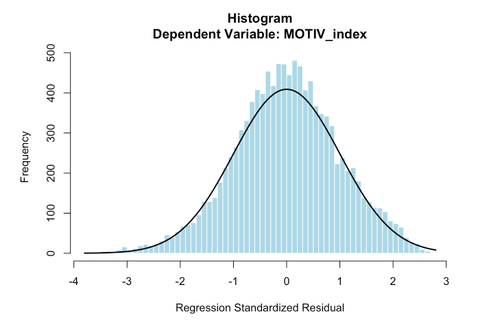
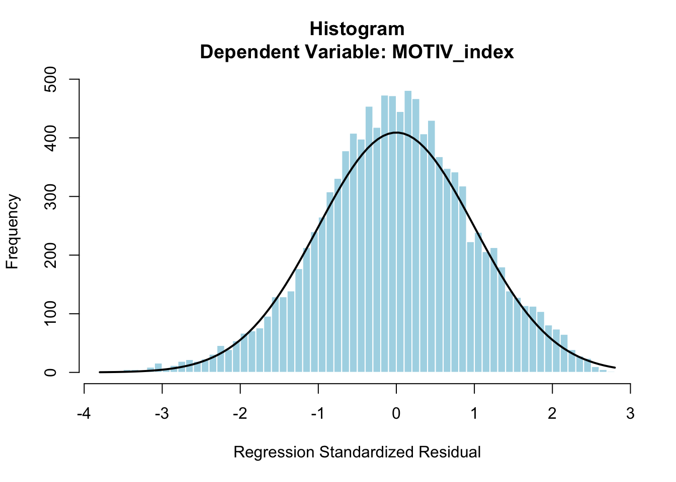
Create Figure 2

hist(rstandard(model3), breaks = 70, col = "lightblue", border = "white",
     main = "Histogram\nDependent Variable: MOTIV_index",
     xlab = "Regression Standardized Residual", ylab = "Frequency")
curve(dnorm(x, mean(rstandard(model3)), sd(rstandard(model3))) * 
        length(rstandard(model3)) * diff(range(rstandard(model3)))/70, add = TRUE, lwd = 2)

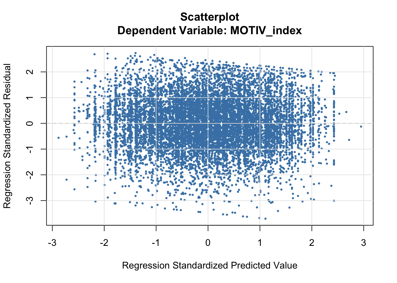
Create Figure 3

std_resid <- rstandard(model3)
std_pred <- scale(fitted(model3))[,1]

plot(std_pred, std_resid,
     main = "Scatterplot\nDependent Variable: MOTIV_index",
     xlab = "Regression Standardized Predicted Value",
     ylab = "Regression Standardized Residual",
     pch = 16, col = "steelblue",  cex = 0.5)    
abline(h = 0, col = "gray50", lty = 2)
grid(col = "gray90", lty = 1)

Table 4 (Correlation Part)

  • Zero-order: simple correlation between predictor and outcome (ignoring other variables)
  • Partial: correlation between predictor and outcome, controlling for all other predictors
  • Part (semi-partial): correlation between predictor and outcome, removing the effect of other predictors from the predictor only
#model1
cor_dt1 <- dt %>% dplyr::select(MOTIV_index, X1PAREDU) %>% mutate(across(everything(), as.numeric)) %>% na.omit()
cor(cor_dt1$MOTIV_index, cor_dt1$X1PAREDU)
[1] 0.1428803
#model2
cor_dt2 <- dt %>% dplyr::select(MOTIV_index, X1PAREDU, P1SCIHWEFF, P1SCICOMP) %>% 
  mutate(across(everything(), as.numeric)) %>% na.omit()
zero_order2 <- cor(cor_dt2)[1, -1]
partial2 <- pcor(cor_dt2)$estimate[1, -1]
part2 <- spcor(cor_dt2)$estimate[1, -1]

data.frame(Variable = names(zero_order2), Zero_order = round(zero_order2, 3),
  Partial = round(partial2, 3),Part = round(part2, 3))
             Variable Zero_order Partial   Part
X1PAREDU     X1PAREDU      0.146   0.126  0.125
P1SCIHWEFF P1SCIHWEFF     -0.102  -0.068 -0.067
P1SCICOMP   P1SCICOMP     -0.024  -0.024 -0.024
#model3
cor_dt3 <- dt %>% dplyr::select(MOTIV_index, X1PAREDU, P1SCIHWEFF, P1SCICOMP, 
                P1MUSEUM, P1COMPUTER, P1FIXED, P1SCIFAIR, P1SCIPROJ, P1STEMDISC) %>%
                mutate(across(everything(), as.numeric)) %>% na.omit()
zero_order3 <- cor(cor_dt3)[1, -1]
partial3 <- pcor(cor_dt3)$estimate[1, -1]
part3 <- spcor(cor_dt3)$estimate[1, -1]

data.frame(Variable = names(zero_order3), Zero_order = round(zero_order3, 3),
  Partial = round(partial3, 3), Part = round(part3, 3))
             Variable Zero_order Partial   Part
X1PAREDU     X1PAREDU      0.145   0.106  0.105
P1SCIHWEFF P1SCIHWEFF     -0.102  -0.051 -0.050
P1SCICOMP   P1SCICOMP     -0.024  -0.021 -0.020
P1MUSEUM     P1MUSEUM      0.090   0.040  0.039
P1COMPUTER P1COMPUTER      0.019  -0.026 -0.025
P1FIXED       P1FIXED      0.048   0.028  0.028
P1SCIFAIR   P1SCIFAIR      0.072   0.033  0.032
P1SCIPROJ   P1SCIPROJ      0.054   0.016  0.016
P1STEMDISC P1STEMDISC      0.124   0.078  0.077

Table 3 ANOVA test

anova(model1, model2, model3)
Analysis of Variance Table

Model 1: MOTIV_index ~ X1PAREDU
Model 2: MOTIV_index ~ X1PAREDU + P1SCIHWEFF + P1SCICOMP
Model 3: MOTIV_index ~ X1PAREDU + P1SCIHWEFF + P1SCICOMP + P1MUSEUM + 
    P1COMPUTER + P1FIXED + P1SCIFAIR + P1SCIPROJ + P1STEMDISC
  Res.Df   RSS Df Sum of Sq      F    Pr(>F)    
1  11150 10782                                  
2  11148 10726  2    56.225 29.627  1.47e-13 ***
3  11142 10573  6   153.100 26.891 < 2.2e-16 ***
---
Signif. codes:  0 '***' 0.001 '**' 0.01 '*' 0.05 '.' 0.1 ' ' 1

4. Brief Methodological Comments on Pinneo & Nolen (2024)

This replication study reveals several methodological ambiguity and concerns that, if addressed, would strengthen the paper’s transparency and reproducibility:

  1. Sample Size Inconsistencies and Missing Data Handling The paper reports multiple sample sizes without clear justification:

    • Initial sample: 24,600 9th graders (HSLS:09 base year)
    • Analysis sample: 14,940 observations
    • Final sample: 14,028 (after removing 7 outliers with |std. residual| > 3)

However, the regression models show different sample sizes without approporate addressing missing values. The replication analysis in Model 3 contains 11,152 observations. The authors should explicitly state whether they used listwise deletion or imputed missing values, and report a single, stable sample size throughout all analyses.

  1. Construction of the Dependent Variable (MOTIV_index)

The paper states that X1SCIID, X1SCIUTI, X1SCIEFF, and X1SCIINT were “created through principal components factor analysis (weighted by W1STUDENT) and standardized to a mean of 0 and a standard deviation of 1” (p. 4). However, the paper does not explain how these four variables were combined into the MOTIV_index composite used as the dependent variable.

The histogram (Figure 2) shows MOTIV_index has mean ≈ 0 and SD = 1.000, suggesting either: (a) it’s a simple mean of already-standardized components, or (b) it was re-standardized after averaging. This ambiguity limits replicability. The authors should could provide a procedure used to create MOTIV_index, including any weighting or standardization steps.

  1. Treatment of Ordinal Variables as Continuous

The regression models treat ordinal categorical variables (parent education levels, parent confidence levels, and gender belief ratings) as continuous numeric predictors without justification or sensitivity testing.

  1. Limited Effect Sizes and Practical Significance

While the paper emphasizes statistical significance (p < 0.001), the effect sizes are notably small. The full model (Model 3) explains only 4% of variance in student science motivation (adjusted R² = 0.038). This raises questions about practical significance and the emphasis on parental factors when 96% of variance remains unexplained.