Social Network Analysis R Tutorial Part 8: Triad Census Models

In this tutorial, we’ll explore triadic structures in social network and their role in understanding social relationships. We’ll learn how to use triad census models within the Tapered ERGM framework to capture complex patterns of transitivity, balance, and clustering in social networks.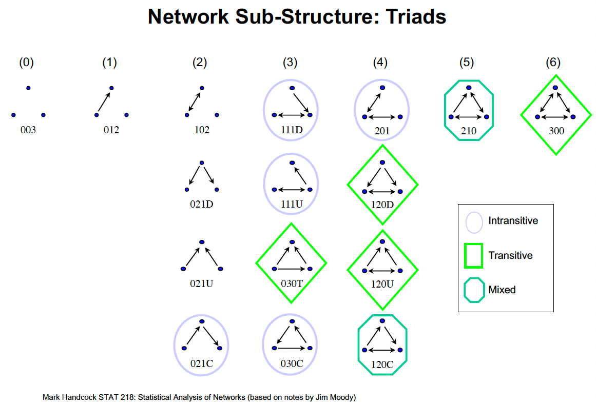

By the end of this tutorial, you’ll understand:

The theoretical foundations of triadic structures and social balance
How to interpret the 16 different triad types in directed networks
How to fit triad census models using ergm.tapered
How to interpret coefficients and evaluate transitivity patterns
How to diagnose convergence and compare competing models

1. Introduction to the Triad Census

1.1 Triad Census Reference Table

**A triad census*

Type	Code	Description	Edges	Pattern (Relationship between A, B, C)
0	003	Empty triad (no ties)	0	A, B, C, empty triad
1	012	One asymmetric tie	1	A $\to$ B, C
2	102	One mutual tie, one null	2	A $\leftrightarrow$ B, C
3	021D	Two asymmetric, “down” pattern	2	A $\leftarrow$ B $\to$ C
4	021U	Two asymmetric, “up” pattern	2	A $\to$ B $\leftarrow$ C
5	021C	Two asymmetric, “cycle”	2	A $\to$ B $\to$ C
6	111D	One mutual, one asymmetric (down)	3	A $\leftrightarrow$ B $\leftarrow$ C
7	111U	One mutual, one asymmetric (up)	3	A $\leftrightarrow$ B $\to$ C
8	030T	Transitive triple (out-star)	3	A $\to$ B $\leftarrow$ C, A $\to$ C
9	030C	Three asymmetric, cyclic	3	A $\leftarrow$ B $\leftarrow$ C, A $\to$ C
10	201	Two mutual, one null	4	A $\leftrightarrow$ B $\leftrightarrow$ C
11	120D	One mutual, two asymmetric (down)	4	A $\leftarrow$ B $\to$ C, A $\leftrightarrow$ C
12	120U	One mutual, two asymmetric (up)	4	A $\to$ B $\leftarrow$ C, A $\leftrightarrow$ C
13	120C	One mutual, two asymmetric (cycle)	4	A $\to$ B $\to$ C, A $\leftrightarrow$ C
14	210	Two mutual, one asymmetric	5	A $\to$ B $\leftrightarrow$ C, A $\leftrightarrow$ C
15	300	Complete (all mutual)	6	A $\leftrightarrow$ B $\leftrightarrow$ C, A $\leftrightarrow$ C, completely connected

Note

Some key transitive patterns to watch for are:

030T: The classic transitive triple (without reciprocation)
120D, 120U: The classic transitive triple (with reciprocation)
300: Complete mutual triangle (ideal balanced triad)
210, 120C: Mixed patterns with transitive closure and reciprocity

2. Model Degeneracy and Tapered ERGMs

2.1 What is Model Degeneracy?

As we mentioned in the SNA tutorial part 6, one challenge in ERGM modeling is near-degeneracy, which occurs when a model places almost all of its probability mass on extreme configurations like:

Empty graphs (no edges)
Complete graphs (all possible edges)
Graphs with no 2-stars
Mono-degree graphs (all nodes have the same degree)

Degeneracy often arises when models include:

High-order structural terms (triangles, k-stars)
Terms that create strong dependencies, such as
Combinations of terms that reinforce extreme structures, such as

Standard ERGMs with triangle terms are particularly prone to degeneracy because triangles create strong positive feedback: more triangles → more edges → even more triangles, leading to nearly complete graphs.

2.2 Tapered ERGM Solution

Beyond using the geometrically-weighted terms, the Tapered ERGM framework (Blackburn & Handcock, 2022) solves the degeneracy problem by adding a “tapering” term that prevents extreme configurations, please check SNA tutorial part 7:

\[q(y|\theta, \tau) = \frac{1}{Z(\theta, \tau)} \exp\left(\sum_k \theta_k g_k(y) - \sum_k \tau_k(\mu_k(\theta, \tau) - g_k(y))^2\right)\]

Note

Practical Interpretation

The tapering term acts like a “spring” that pulls the model away from extreme configurations. The strength of this spring ($\tau$) is automatically calibrated to ensure model stability while preserving the effects of the structural terms.

3. Example 1: Modeling a Triad Census in Hansell Classroom Friendship Network

Here we consider again the network introduced in SNA tutorial part 5 of strong friendship ties among 13 boys and 14 girls in a sixthgrade classroom, as collected by Hansell (1984). Each student was asked if they liked each other student “a lot”, “some”, or “not much”. Here we consider a strong friendship tie to exist if a student likes another student “a lot.” Also recorded is the sex of each student. The data is in the networkdata package.

Code

rm(list = ls())

#install.packages("ergm", repos="http://www.stat.ucla.edu/~handcock")
#install.packages("ergm.tapered", repos="http://www.stat.ucla.edu/~handcock")
#or devtools::install_github("statnet/ergm.tapered")
#devtools::install_github('statnet/ergm', ref='tapered')
#install.packages("ergm.tapered")

library(networkdata)
library(network)
library(ergm)
library(sna)
library(ergm.tapered)

3.1 Fit a triad census model using ergm.tapered. Include a term for homophily by sex.

Code

data("hansell")
help(hansell)
table(hansell %v% "sex")


female   male 
    14     13

Code

sex_attr <- hansell %v% "sex"
vertex_colors <- ifelse(sex_attr == "male", "lightblue", "lightpink")

set.seed(42)
plot(hansell,
     vertex.col = vertex_colors,
     main = "Hansell Classroom Friendship Network",
     vertex.cex = 2,
     label = 1:network.size(hansell),
     label.cex = 0.8)

legend("topright",
       legend = c("Male", "Female"),
       col = c("lightblue", "lightpink"),
       pch = 19,
       pt.cex = 2)

Code

triad.census(hansell)

     003 012 102 021D 021U 021C 111D 111U 030T 030C 201 120D 120U 120C 210 300
[1,] 771 982 248  234  115  150   68   97  126    2  13   32   32   20  28   7

Code

triad.census(hansell)[2]

[1] 982

Code

set.seed(42)
fit1a <- ergm.tapered(hansell ~ edges + nodematch("sex") + triadcensus(c(1:8, 10:15)),
                      control = control.ergm.tapered(seed = 123))
summary(fit1a)

 Results:

                 Estimate Std. Error MCMC % z value Pr(>|z|)    
edges            -12.1760     5.8895      0  -2.067 0.038694 *  
nodematch.sex      0.9125     0.2650      0   3.444 0.000573 ***
triadcensus.012    0.3406     0.2335      0   1.459 0.144605    
triadcensus.102    0.8071     0.4695      0   1.719 0.085617 .  
triadcensus.021D   0.8390     0.4703      0   1.784 0.074442 .  
triadcensus.021U   0.8016     0.4650      0   1.724 0.084755 .  
triadcensus.021C   0.7018     0.4805      0   1.461 0.144125    
triadcensus.111D   1.0480     0.7126      0   1.471 0.141387    
triadcensus.111U   1.1019     0.7076      0   1.557 0.119436    
triadcensus.030T   1.4666     0.7089      0   2.069 0.038570 *  
triadcensus.201    1.4035     0.9545      0   1.470 0.141448    
triadcensus.120D   1.8346     0.9378      0   1.956 0.050426 .  
triadcensus.120U   1.9169     0.9358      0   2.049 0.040508 *  
triadcensus.120C   1.5512     0.9756      0   1.590 0.111848    
triadcensus.210    2.3795     1.1754      0   2.024 0.042932 *  
triadcensus.300    3.5463     1.4308      0   2.478 0.013195 *  
---
Signif. codes:  0 '***' 0.001 '**' 0.01 '*' 0.05 '.' 0.1 ' ' 1
The estimated tapering scaling factor is 2.

     Null Deviance: 973.2  on 702  degrees of freedom
 Residual Deviance: 653.1  on 686  degrees of freedom
 
AIC: 685.1  BIC: 758  (Smaller is better. MC Std. Err. = 0)

Code

coef_table1a <- data.frame(
  Coefficient = round(coef(fit1a), 3),
  SE = round(summary(fit1a)$coefficients[, "Std. Error"], 3),
  OR = round(exp(coef(fit1a)), 3),
  p_value = round(summary(fit1a)$coefficients[, "Pr(>|z|)"], 4)
)

print(coef_table1a)

                 Coefficient    SE     OR p_value
edges                -12.176 5.889  0.000  0.0387
nodematch.sex          0.913 0.265  2.491  0.0006
triadcensus.012        0.341 0.233  1.406  0.1446
triadcensus.102        0.807 0.470  2.241  0.0856
triadcensus.021D       0.839 0.470  2.314  0.0744
triadcensus.021U       0.802 0.465  2.229  0.0848
triadcensus.021C       0.702 0.481  2.017  0.1441
triadcensus.111D       1.048 0.713  2.852  0.1414
triadcensus.111U       1.102 0.708  3.010  0.1194
triadcensus.030T       1.467 0.709  4.334  0.0386
triadcensus.201        1.403 0.954  4.069  0.1414
triadcensus.120D       1.835 0.938  6.262  0.0504
triadcensus.120U       1.917 0.936  6.800  0.0405
triadcensus.120C       1.551 0.976  4.717  0.1118
triadcensus.210        2.379 1.175 10.799  0.0429
triadcensus.300        3.546 1.431 34.684  0.0132

Code

plogis(coef(fit1a)["edges"] + coef(fit1a)["nodematch.sex"])

       edges 
1.283287e-05

3.2 Interpretation

Edges: $\beta = -12.18**$ represents the baseline log-odds of a friendship tie exisiting between any two randomly selected students in the network, while controlling for other predictors. The $OR=0.00$, means the baseline odds of a tie is very very small.
Nodematch.sex: $\beta = 0.91***$ represents the additional log-odds of a friendship tie when both students are of the same sex, relative to cross-sex friendships. The positive and highly significant coefficient indicates strong homophily by sex. The $OR = 2.49$ means same-sex friendships are about 2.49 times more likely than cross-sex friendships, holding all else constant. There is homophily by sex.
Triad Census Terms (relative to empty triads - 003):
- Transitive Patters (300, 120D, 030T, 120U):
  - triadcensus.030T: $\beta = 1.47*$. The classic transitive triple where (without reciprocation). The positive and significant coefficient indicates strong transitivity preference. The $OR = exp(1.47) = 4.33$ means transitive triples are 4.35 times more likely than empty triads. This is the “friend of friend is friend” pattern.
  - triadcensus.300: $\beta = 3.55*$. Complete mutual triangle where all three pairs are friends with full reciprocity (significant). The $OR = 34.81$ means complete triangles are nearly 35 times more likely than empty triads. This provides theevidence of transitive closure and represents the ideal balanced triad in structural balance theory.
  - triadcensus.120D: $\beta = 1.83$. One mutual ties plus two down asymmetric tie. The $OR = 6.23$.
  - triadcensus.120U: $\beta = 1.92*$. Similar transitive pattern with one mutual ties and two up asymmetric ties (significant). The $OR = 6.80$. Like 120D, this shows strong transitive closure with reciprocity.
  - Based on these patterns, there is a general preference for transitive friendship ties.
- Intransitive Patterns (111D, 201, 111U, 021C, 030C):
  - Null of the intransitive patterns triadcensus coefficient is signification. There is no strong evidence to show that the network is intransitive.

4. Example 2: Modeling a Triad Census in Grade 9 Girls Friendship Network

Now let’s analyze a different dataset: friendships among 9th grade girls.

Source: gfriends dataset from networkdata
We’ll extract only grade 9 students
Node attributes: GPA and smoking behavior
Directed network

Research Questions:

How do individual attributes (GPA, smoking) affect friendship formation?
What triadic patterns characterize this friendship network?
Can we find a simpler, more fitness model?

Code

suppressMessages(library(networkdata)) #just loads silently
data(gfriends)
help(gfriends)

4.1 Fit a triad census model

First, extract out the grade nine students using gfriends$X[,1]==9 and create a directed network. Also add a vertex variable equal to the student gpa.

Fit a triad census model using a subset of the first seven triad types (012, 102, 021D, 021U, 021C, 111D, 111U). Recall that 003 is the reference category. Also include GPA and smoking effects, using something like:

Code

head(gfriends[["X"]])

     grade   gpa smoke
[1,]    11 -1.20  1.38
[2,]    10  1.83 -0.40
[3,]    10  0.89  2.17
[4,]    11 -0.25  0.33
[5,]    12  1.23  0.99
[6,]    12  1.68 -0.18

Code

#extract the 9th grade student
grade9_idx <- which(gfriends$X[, 1] == 9)
head(gfriends$X[grade9_idx, ])

     grade   gpa smoke
[1,]     9  1.70  1.22
[2,]     9 -0.53  0.37
[3,]     9  0.77 -0.93
[4,]     9  0.05  0.58
[5,]     9  0.77  0.41
[6,]     9  1.93 -0.84

Code

length(grade9_idx)

[1] 29

Code

gf_matrix <- gfriends$Y[grade9_idx, grade9_idx]
dim(gf_matrix)

[1] 29 29

Code

#create the network object
gf <- network(gf_matrix, directed = TRUE)

#add vertex attributes
gf %v% "gpa" <- gfriends$X[grade9_idx, 2]
gf %v% "smoke" <- gfriends$X[grade9_idx, 3]

#fit model
fit2a <- ergm.tapered(gf ~ edges + nodecov("gpa") + nodecov("smoke") + triadcensus(c(1:7)),
                      control = control.ergm.tapered(seed = 123))
summary(fit2a)

 Results:

                 Estimate Std. Error MCMC % z value Pr(>|z|)  
edges            -1.80740    1.27939      1  -1.413   0.1577  
nodecov.gpa       0.18903    0.09563      1   1.977   0.0481 *
nodecov.smoke    -0.24255    0.11483      2  -2.112   0.0347 *
triadcensus.012  -0.00433    0.06225      1  -0.070   0.9445  
triadcensus.102   0.04837    0.12451      1   0.388   0.6977  
triadcensus.021D -0.87374    0.36572      0  -2.389   0.0169 *
triadcensus.021U  0.14984    0.11155      1   1.343   0.1792  
triadcensus.021C -0.33749    0.21167      1  -1.594   0.1108  
triadcensus.111D -0.11008    0.18176      1  -0.606   0.5448  
triadcensus.111U -0.44240    0.23456      0  -1.886   0.0593 .
---
Signif. codes:  0 '***' 0.001 '**' 0.01 '*' 0.05 '.' 0.1 ' ' 1
The estimated tapering scaling factor is 2.

     Null Deviance: 1125.7  on 812  degrees of freedom
 Residual Deviance:  420.1  on 802  degrees of freedom
 
AIC: 440.1  BIC: 487  (Smaller is better. MC Std. Err. = 0)

Code

coef_table2a <- data.frame(
  Coefficient = round(coef(fit2a), 3),
  SE = round(summary(fit2a)$coefficients[, "Std. Error"], 3),
  OR = round(exp(coef(fit2a)), 3),
  p_value = round(summary(fit2a)$coefficients[, "Pr(>|z|)"], 4)
)

print(coef_table2a)

                 Coefficient    SE    OR p_value
edges                 -1.807 1.279 0.164  0.1577
nodecov.gpa            0.189 0.096 1.208  0.0481
nodecov.smoke         -0.243 0.115 0.785  0.0347
triadcensus.012       -0.004 0.062 0.996  0.9445
triadcensus.102        0.048 0.125 1.050  0.6977
triadcensus.021D      -0.874 0.366 0.417  0.0169
triadcensus.021U       0.150 0.112 1.162  0.1792
triadcensus.021C      -0.337 0.212 0.714  0.1108
triadcensus.111D      -0.110 0.182 0.896  0.5448
triadcensus.111U      -0.442 0.235 0.642  0.0593

Code

plogis(coef(fit2a)["edges"])

    edges 
0.1409529

Code

plogis(coef(fit2a)["edges"] + coef(fit2a)["nodecov.gpa"])

    edges 
0.1654296

4.2 Interpretation

Edges: $\beta= -1.81$ Represents the baseline log-odds of a friendship tie existing between any two randomly selected grade 9 girls in the network, while controlling for GPA, smoking behavior, and triad configurations. The negative coefficient indicates the network is sparse, though the effect is not statistically significant. The $OR = exp(-1.81) = 0.164$ means the baseline odds of a tie is about 16.4%. The baseline probability of friendship is approximately $plogis(-1.81) = 14.1%$. The non-significance suggests that once we account for individual attributes (GPA, smoking) and structural patterns (triad census), the baseline density is not significantly different from what would be expected.
Nodecov.gpa: $\beta= 0.19*$ Represents the change in log-odds of sending or receiving a friendship tie for each one standard deviation increase in GPA. The positive and significant coefficient indicates that students with higher GPAs are more active in the friendship network. The $OR = exp(0.19) = 1.21$ means that for each unit increase in GPA, a student is 1.21 times more likely to be involved in friendship ties (either sending or receiving). This could reflect either greater social engagement among high-achieving students, or that academically successful students are more sought after as friends, or both.
Nodecov.smoke: $\beta= -0.24*$ Represents the change in log-odds of sending or receiving a friendship tie associated with smoking behavior. The negative and significant coefficient indicates that students who smoke are less active in the friendship network. The $OR = exp(-0.24) = 0.79$ means that smokers are about 0.79 times as likely to be involved in friendship ties compared to non-smokers, or equivalently, they have about 21% lower odds of friendship activity. This could reflect social marginalization of smokers, or that smokers form smaller, more selective friendship groups.
Triad Census Terms (relative to empty triads, type 003):
triadcensus.021D: $\beta= -0.87*$. The “triadic out-star” pattern where one student send out two ties to two others who are not connected. The negative and significant coefficient has $OR = 0.42$ means these patterns are only 42% as likely as empty triads, they are significantly under-represented. This suggests the network actively avoids asymmetric popularity structures where one person is the focus of attention without reciprocation or closure.

4.3 MCMC diagnostic

Look at the MCMC diagnostics for the model (via, e.g., mcmc.diagnostics(fit)). What does it say about the convergence of the model?

The model has converged sufficiently for preliminary analysis, but several diagnostics indicate room for improvement. The overall Chi-squared test (p = 0.039) is marginally significant, suggesting some discrepancy between sample and observed statistics. The concerning terms include: nodecov.smoke, triadcensus.102, and triadcensus.021C.

Code

mcmc.diagnostics(fit2a)

Sample statistics summary:

Iterations = 8704:163840
Thinning interval = 512 
Number of chains = 1 
Sample size per chain = 304 

1. Empirical mean and standard deviation for each variable,
   plus standard error of the mean:

                     Mean     SD Naive SE Time-series SE
edges            -0.14803  2.999   0.1720         0.1720
nodecov.gpa       0.13115  8.423   0.4831         0.7120
nodecov.smoke    -0.41757  3.706   0.2125         0.2125
triadcensus.012   1.78618 29.233   1.6766         1.6766
triadcensus.102  -3.08882 22.878   1.3121         1.4401
triadcensus.021D  0.03618  2.121   0.1216         0.1216
triadcensus.021U -0.44737  5.137   0.2946         0.2946
triadcensus.021C  0.50000  3.747   0.2149         0.2149
triadcensus.111D -0.52632  6.082   0.3488         0.3488
triadcensus.111U -0.36842  3.470   0.1990         0.1990

2. Quantiles for each variable:

                    2.5%     25%    50%    75%  97.5%
edges             -6.000  -2.000  0.000  2.000  5.000
nodecov.gpa      -15.553  -5.577 -0.120  6.343 15.565
nodecov.smoke     -6.871  -3.002 -0.535  2.013  6.634
triadcensus.012  -48.425 -19.000  2.000 21.000 61.000
triadcensus.102  -52.000 -19.000 -4.000 11.000 40.850
triadcensus.021D  -4.000  -1.000  0.000  1.000  5.000
triadcensus.021U  -9.000  -4.000 -1.000  3.000 10.000
triadcensus.021C  -6.425  -2.000  0.000  3.000  8.000
triadcensus.111D -11.425  -5.000 -0.500  3.000 12.000
triadcensus.111U  -6.425  -3.000  0.000  2.000  7.000


Are sample statistics significantly different from observed?
                edges nodecov.gpa nodecov.smoke triadcensus.012 triadcensus.102
diff.      -0.1480263   0.1311513   -0.41756579       1.7861842      -3.0888158
test stat. -0.8607291   0.1842048   -1.96470916       1.0653334      -2.1449155
P-val.      0.3893873   0.8538528    0.04944791       0.2867251       0.0319596
           triadcensus.021D triadcensus.021U triadcensus.021C triadcensus.111D
diff.            0.03618421       -0.4473684       0.50000000       -0.5263158
test stat.       0.29750393       -1.5184829       2.32664095       -1.5088446
P-val.           0.76608181        0.1288927       0.01998438        0.1313385
           triadcensus.111U Overall (Chi^2)
diff.           -0.36842105              NA
test stat.      -1.85110594     20.36452347
P-val.           0.06415431      0.03869803

Sample statistics cross-correlations:
                      edges nodecov.gpa nodecov.smoke triadcensus.012
edges             1.0000000  0.37889013  -0.127881804     0.433521974
nodecov.gpa       0.3788901  1.00000000  -0.079132618     0.097116160
nodecov.smoke    -0.1278818 -0.07913262   1.000000000     0.000792673
triadcensus.012   0.4335220  0.09711616   0.000792673     1.000000000
triadcensus.102   0.7231911  0.23804490  -0.008926377    -0.167756780
triadcensus.021D  0.1809454  0.06405166  -0.124792118     0.229099184
triadcensus.021U  0.1838132  0.11110899   0.019262822     0.247668056
triadcensus.021C  0.1761002  0.05621847   0.053913541     0.168684089
triadcensus.111D  0.5274072  0.21140965  -0.122677466     0.248699177
triadcensus.111U  0.2167637  0.04946134  -0.006336053     0.103653234
                 triadcensus.102 triadcensus.021D triadcensus.021U
edges                0.723191072      0.180945405       0.18381316
nodecov.gpa          0.238044902      0.064051657       0.11110899
nodecov.smoke       -0.008926377     -0.124792118       0.01926282
triadcensus.012     -0.167756780      0.229099184       0.24766806
triadcensus.102      1.000000000      0.009386180      -0.09871617
triadcensus.021D     0.009386180      1.000000000       0.10177455
triadcensus.021U    -0.098716174      0.101774551       1.00000000
triadcensus.021C     0.002444791      0.005191905       0.05075507
triadcensus.111D     0.212996725      0.171905078       0.16389140
triadcensus.111U     0.149742658     -0.162326583       0.06422630
                 triadcensus.021C triadcensus.111D triadcensus.111U
edges                 0.176100215       0.52740722      0.216763684
nodecov.gpa           0.056218472       0.21140965      0.049461337
nodecov.smoke         0.053913541      -0.12267747     -0.006336053
triadcensus.012       0.168684089       0.24869918      0.103653234
triadcensus.102       0.002444791       0.21299673      0.149742658
triadcensus.021D      0.005191905       0.17190508     -0.162326583
triadcensus.021U      0.050755072       0.16389140      0.064226302
triadcensus.021C      1.000000000      -0.05286085      0.114220091
triadcensus.111D     -0.052860850       1.00000000     -0.090376816
triadcensus.111U      0.114220091      -0.09037682      1.000000000

Sample statistics auto-correlation:
Chain 1 
               edges nodecov.gpa nodecov.smoke triadcensus.012 triadcensus.102
Lag 0     1.00000000   1.0000000   1.000000000     1.000000000     1.000000000
Lag 512   0.06739725   0.3680833   0.065623895    -0.048041725     0.091133350
Lag 1024  0.05825373   0.1646531   0.015884782    -0.011485501     0.002775281
Lag 1536 -0.01469089   0.1178725   0.098920723     0.065961612     0.030321197
Lag 2048  0.09159919   0.1367854   0.063744152     0.001694241    -0.025794569
Lag 2560  0.07722141   0.1708562  -0.008474055    -0.014118546     0.038911850
         triadcensus.021D triadcensus.021U triadcensus.021C triadcensus.111D
Lag 0          1.00000000     1.0000000000      1.000000000       1.00000000
Lag 512       -0.07819163     0.0536258615      0.041549130      -0.06008633
Lag 1024       0.08114121     0.0747122912     -0.011283498       0.06508384
Lag 1536      -0.06120786     0.0337710463      0.042019276      -0.07208703
Lag 2048      -0.06639916    -0.0416285550     -0.002820874       0.09375034
Lag 2560       0.02324068    -0.0003621479      0.092324871       0.01138627
         triadcensus.111U
Lag 0          1.00000000
Lag 512       -0.02225109
Lag 1024      -0.02756769
Lag 1536      -0.02802321
Lag 2048      -0.04629310
Lag 2560       0.01210376

Sample statistics burn-in diagnostic (Geweke):
Chain 1 

Fraction in 1st window = 0.1
Fraction in 2nd window = 0.5 

           edges      nodecov.gpa    nodecov.smoke  triadcensus.012 
         -0.3218          -0.1302           0.8133          -0.3304 
 triadcensus.102 triadcensus.021D triadcensus.021U triadcensus.021C 
         -1.1369           0.2882           0.1211           3.0275 
triadcensus.111D triadcensus.111U 
          0.6998           0.7543 

Individual P-values (lower = worse):
           edges      nodecov.gpa    nodecov.smoke  triadcensus.012 
     0.747633943      0.896404640      0.416026288      0.741086904 
 triadcensus.102 triadcensus.021D triadcensus.021U triadcensus.021C 
     0.255566303      0.773219437      0.903595250      0.002465625 
triadcensus.111D triadcensus.111U 
     0.484043549      0.450683666 
Joint P-value (lower = worse):  0.4441709 .


MCMC diagnostics shown here are from the last round of simulation, prior to computation of final parameter estimates. Because the final estimates are refinements of those used for this simulation run, these diagnostics may understate model performance. To directly assess the performance of the final model on in-model statistics, please use the GOF command: gof(ergmFitObject, GOF=~model).

4.4 Model Comparison

Try to fit a model with fewer terms than that in a). What is the preferred model?

The model with fewer terms have better fitness.The simple model with only 2 triad types (012, 102) is the preferred model, as it has the lowest AIC (437.08) and BIC (460.58) compared to the reduced model (AIC: 438.61, BIC: 471.50) and full model (AIC: 440.05, BIC: 487.05). This suggests that the additional triad census terms (types 3-7) do not provide sufficient explanatory power to justify their added complexity, and the network structure is adequately captured by individual attributes (GPA, smoking) and the simplest asymmetric and reciprocated dyad patterns.

Code

fit2d_1 <- ergm.tapered(gf ~ edges + nodecov("gpa") + nodecov("smoke") + triadcensus(c(1:4)))

fit2d_2 <- ergm.tapered(gf ~ edges + nodecov("gpa") + nodecov("smoke") + triadcensus(c(1, 2)))

cat(sprintf("Full model (7 triad types) AIC: %.2f, BIC: %.2f\n", AIC(fit2a), BIC(fit2a)))

Full model (7 triad types) AIC: 440.05, BIC: 487.05

Code

cat(sprintf("Reduced model (4 triad types) AIC: %.2f, BIC: %.2f\n", AIC(fit2d_1), BIC(fit2d_1)))

Reduced model (4 triad types) AIC: 438.61, BIC: 471.50

Code

cat(sprintf("Simple model (2 triad types) AIC: %.2f, BIC: %.2f\n", AIC(fit2d_2), BIC(fit2d_2)))

Simple model (2 triad types) AIC: 437.08, BIC: 460.58

This tutorial is based on UCLA STATS 218: Social Network Analysis taught by Prof Mark Handcock.